Longitudinal Fecal Calprotectin Profiles Characterize Disease Course Heterogeneity in Crohn’s Disease

set.seed(123)

# Fitting the LCMMs takes around three hours (when running single threaded)
# if cache.models is true then the saved model objects will be used instead of
# refitting the models
cache.models <- TRUE

##########################
#--     Packages       --#
##########################

library(tidyverse)
## Modelling ##
library(lcmm)
library(splines)
## Presentation ##
library(htmltools)
library(patchwork)
library(ggdist)
library(grid)
library(ggalluvial)
library(qqplotr)

if (!require(DT)) {
  install.packages("DT")
}

##########################
#--     Data read      --#
##########################

FCcumulative <- readRDS(paste0("/Volumes/igmm/cvallejo-predicct/",
                               "cdi/processed/",
                               "FCcumulativeLongInc.RDS")
                        )

###########################################
#-- Create directories and readme files --#
###########################################

if (!dir.exists("plots")) {
  dir.create("plots")
}

fileConn <- file("plots/README.md")
writeLines(c("# README",
             "",
             paste("This directory contains plots created by the analysis", 
                   "but are not provided as figures (supplementary or", 
                   "otherwise) in the paper")),
           fileConn)
close(fileConn)


if (!dir.exists("cache")) dir.create("cache")
fileConn <- file("cache/README.md")
writeLines(c("# README",
             "",
             paste("This directory stores cached versions of R objects which",
                   "take a long time to create (such as LCMM fit objects).")),
           fileConn)
close(fileConn)

if (!dir.exists("paper")) dir.create("paper")
fileConn <- file("paper/README.md")
writeLines(c("# README",
             "",
             paste("This directory contains all figures used in the paper.",
                   "The sup subdirectory contains supplementary figures")),
           fileConn)
close(fileConn)

if (!dir.exists("paper/sup")) dir.create("paper/sup")

if (!dir.exists("plots/residuals")) {
  dir.create("plots/residuals")
}

########################
#-- Custom Functions --#
########################

# Build DT::datatable objects from matrix of fit statistics
DTbuild <- function(hlme.metric, caption) {
  hlme.metrics <- cbind(hlme.metrics, group = seq(1, nrow(hlme.metrics)))
  hlme.metrics <- hlme.metrics[, c(4, 1, 2, 3)]
  DT::datatable(round(as.data.frame(hlme.metrics), 2),
                options = list(dom = 't'),
                caption = tags$caption(
                  style = 'text-align: center;',
                  h3(caption)),
                style ="bootstrap4",
                rownames = FALSE,
                colnames = c("Clusters",
                             "Maximum log-likelihood",
                             "AIC",
                             "BIC"),
                escape = FALSE)
}

#' Spaghetti plots of each class
#' @param models list containing HLME objects
#' @param G How many classes does the model assume?
#' @param log Logical. Should plots be on log scale
#' @param indi Logical. Should separate plots for each class be generated?
#' @param multi Logical. Should all plots be plotted alongside each other? 
#' @param tmax Maximum observation period
#' @param column Logical. Should all sub-plots be in a single column? Defaults
#'   to false (two columns)
#' @param prob.cutoff Posterior probability cut-off for subjects to be included
#'   as trajectories
#' @param mapping Numeric vector which gives reordering of plots in a
#'   multiplot. Need to take into account plots are generated by column - not
#'   row
#' @param sizes Output latent class sizes
#' @param save Logical. Should sub figure labels be generated?
spaghetti_plot <- function(FCcumulative,
                           models,
                           G,
                           log = TRUE,
                           indi = FALSE, 
                           multi = TRUE,
                           tmax = 5,
                           column =  FALSE, 
                           pprob.cutoff = NA,
                           sizes = FALSE,
                           mapping = NULL,
                           save = FALSE){
  
  if(!is.na(pprob.cutoff)) {
    pprob.cutoffs <- c()
    
    for (subject in unique(models[[G]]$pprob$id)){
      temp <- subset(models[[G]]$pprob, id == subject)
      pprob <- temp[, 2 + temp$class]
      if (pprob > pprob.cutoff) {
        pprob.cutoffs <- c(pprob.cutoffs, subject)
      }
    }
    FCcumulative <- subset(FCcumulative, id %in% pprob.cutoffs)
  }
  
  if (indi){
    spaghetti_plot_sub(FCcumulative = FCcumulative, 
                       models = models,
                       G = G,
                       log = log,
                       multi = FALSE,
                       tmax = tmax,
                       column = column,
                       pprob = pprob,
                       sizes = sizes,
                       mapping = mapping)
    }
  if (multi){
      spaghetti_plot_sub(FCcumulative = FCcumulative, 
                         models = models,
                         G = G,
                         log = log,
                         multi = TRUE,
                         tmax = tmax,
                         column = column,
                         pprob = pprob,
                         sizes = sizes,
                         mapping = mapping,
                         save = save)
  }
}

spaghetti_plot_sub <- function(FCcumulative,
                           models,
                           G,
                           multi = FALSE,
                           log,
                           unit,
                           tmax = 5,
                           column = column,
                           pprob = NA,
                           sizes = sizes,
                           mapping = mapping,
                           save = save){
  
  labels <- c("A", "C", "B", "D")
  
  time <- seq(0, tmax, by = 0.01)
  
  if (column) {
    # use single column layout for sub-plots
    layout <- matrix(seq(1, G),
                   ncol = 1,
                   nrow = G)
  } else {
    # use two column layout for sub-plots
      layout <- matrix(seq(1, 2 * ceiling(G / 2)),
                   ncol = 2,
                   nrow = ceiling(G / 2))
  }
  # Set up the page
  pushViewport(viewport(layout = grid.layout(nrow(layout), ncol(layout))))
  
  data_pred <- data.frame(time = time)
  pred <- predictY(models[[G]],
                   data_pred,
                   var.time = "time",
                   draws = TRUE)
  lcmm_uit <- as.data.frame(pred$pred)
  lcmm_uit$time <- time
  
  if(is.null(mapping)) {
    mapping <- 1:G
  }
  
  
  for (g in mapping) {
    matchidx <- as.data.frame(which(layout == g, arr.ind = TRUE))
    id.group <- models[[G]]$pprob[models[[G]]$pprob[, 2] == mapping[g], 1]
    if (sizes) {
      message("There are ",
              length(id.group),
              " subjects in cluster ",
              g,
              ".")
    }
    if(!log){
      p[[g]] <- ggplot(data = subset(FCcumulative, id %in% id.group),
                     aes(x = time, y = exp(value))) +
      geom_line(aes(group = id), alpha = 0.1) +
      theme_minimal() + 
      geom_line(data = lcmm_uit,
                aes(x = time,
                    y = exp(lcmm_uit[, paste0("Ypred_class", mapping[g])])),
                size = 1.5,
                col = "red") +
      geom_line(data = lcmm_uit,
                aes(x = time,
                    y = exp(lcmm_uit[, paste0("lower.Ypred_class",
                                              mapping[g])])),
                col = "red",
                lty = 2) +
      geom_line(data = lcmm_uit,
                aes(x = time,
                    y = exp(lcmm_uit[, paste0("upper.Ypred_class",
                                              mapping[g])])),
                col = "red",
                lty = 2) +
      xlab("Time (years)") +
      ylab("FCAL (μg/g)") +
      ylim(0, 2500)
    } else{
       p[[g]] <- ggplot(data = subset(FCcumulative, id %in% id.group),
                     aes(x = time, y = value)) +
      geom_line(aes(group = id), alpha = 0.1) +
      theme_minimal() + 
      geom_line(data = lcmm_uit,
                aes(x = time, y = lcmm_uit[, paste0("Ypred_class",
                                                    mapping[g])]),
                size = 1.5,
                col = "red") +
      geom_line(data = lcmm_uit,
                aes(x = time, y = lcmm_uit[, paste0("lower.Ypred_class",
                                                    mapping[g])]),
                col = "red",
                lty = 2) +
      geom_line(data = lcmm_uit,
                aes(x = time, y = lcmm_uit[, paste0("upper.Ypred_class",
                                                    mapping[g])]),
                col = "red",
                lty = 2) +
      geom_hline(yintercept = log(250),
                 color = "#007add",
                 lty = 3,
                 size = 1.5) +
      xlab("Time (years)") +
      ylab("Log (FCAL (μg/g))") +
      ylim(2, log(2500))
    }
    if (multi) {
      if (save) {
        # Add subfigure labels
        print(p[[g]] +
                ggtitle(labels[g]) +
                theme_classic() +
                theme(axis.line = element_line(colour = "gray"),
                      plot.title = element_text(face = "bold",
                                                size = 20)),
              vp = viewport(layout.pos.row = matchidx$row,
                            layout.pos.col = matchidx$col)
              )
      } else {
        print(p[[g]],
              vp = viewport(layout.pos.row = matchidx$row,
                            layout.pos.col = matchidx$col)
              )
      }
    } else {
      print(p[[g]])
    }
  }
}

To achieve our aims of identifying clusters within the CD population with similar FCAL profiles, we use latent class mixed models (LCMMs) with natural cubic spline formulations for the fixed and random effects components. LCMMs are an extension of linear mixed effects models with an added fixed effect class-specific component. Cluster membership in a LCMM is given via a multinomial logistic model.

Previously, we have investigated using polynomial regression models with an I-splines link function, and models which use Gaussian radial basis functions (GRBFs) in order to model the fixed and random components of an LCMM. Unfortunately, the polynomial regression and I-splines link approaches demonstrated inflexibility and, in the case of polynomial regression behaved erratically near the ends of the time period.

The GRBF approach was very sensitive to l, a length scale parameter, and the iterative Marquardt algorithm implemented in the lcmm package did not converge in many cases- possibly due the number of parameters required to be estimated and/or the Runge phenomenon (Fornberg and Zuev 2007).

This has led us to consider an approach using natural cubic splines which has a few notable advantages (Elhakeem et al. 2022):

Less parameters need to be estimated than either a Gaussian radial basis function regression model or a polynomial regression model with the same flexibility . This reduces the time complexity when fitting the model and in the future may also make extensions more practically feasible.
Natural cubic splines enforce linearity between t_0 and the first knot and between the last knot and t_\text{max} which ensures the model does not behave erratically in these sometimes problematic areas.
Natural cubics are not highly sensitive to a continuous parameter and instead requires only K, the number of knots, to be tuned: being robust to where the knots themselves are placed.

Formal defintions

For formal definitions of the models and statistics we have used in the work, please see the supplementary material for our paper.

The Crohn’s Disease Inception Cohort

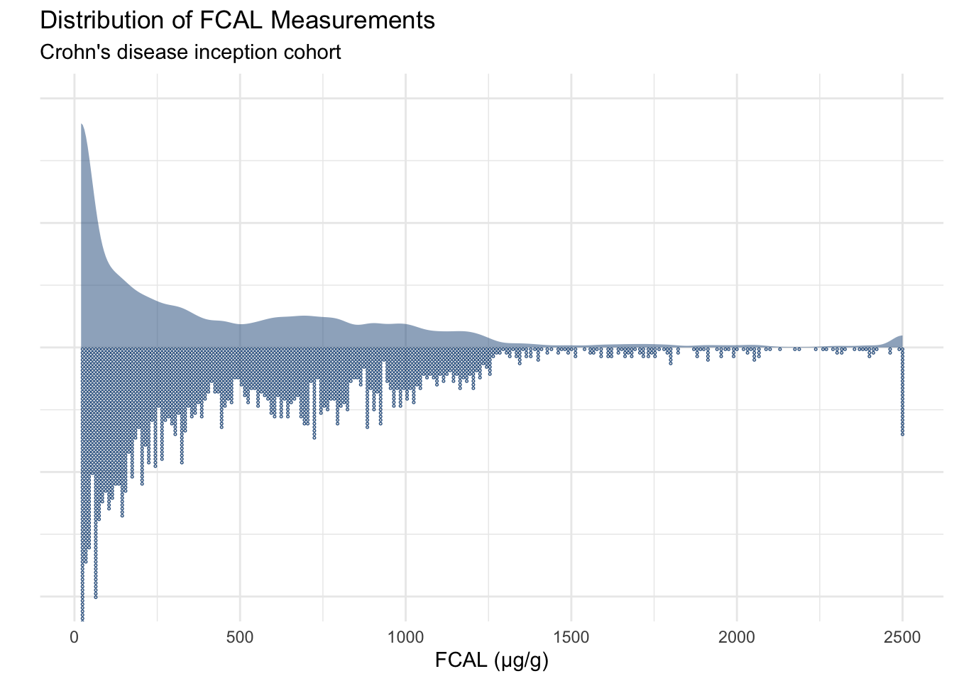
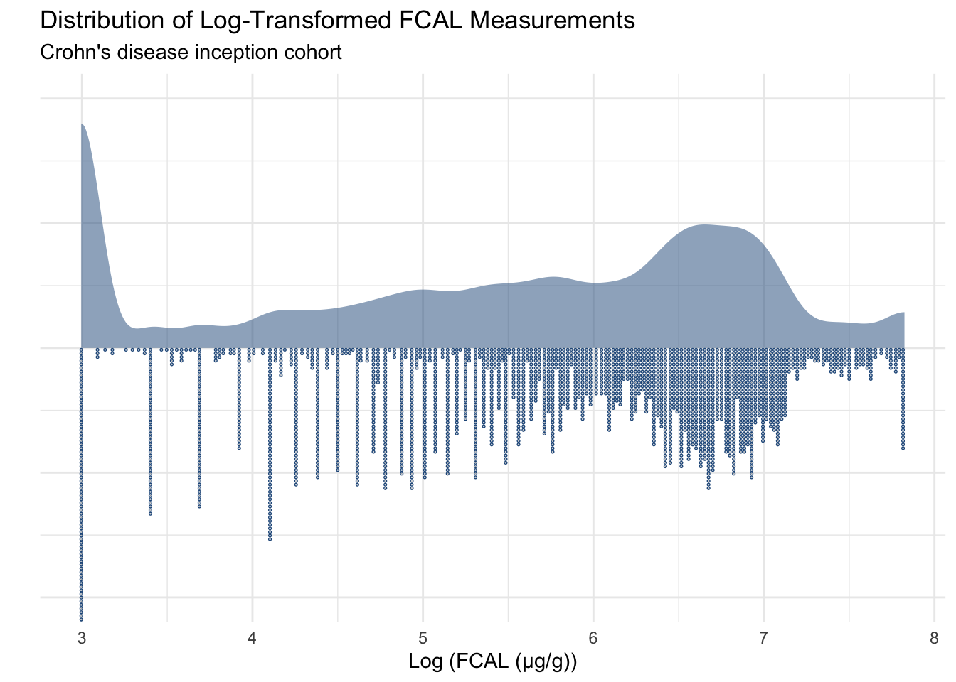
The background for the data we will fit to the models and an explanation of the data processing steps implemented can be found on a dedicated page. Due to the distribution of the FCAL values (Figure 1), FCAL values have been log-transformed prior to model fitting (Figure 2).

Code

FCcumulative %>%
  ggplot(aes(x = value, y = NULL)) +
  stat_slab(size = 0.8, alpha = 0.5, fill = "#235789") +
  geom_dots(binwidth = 10, size = 1, side = "bottom", color = "#235789") +
  theme_minimal() +
  theme(axis.text.y = element_blank()) +
  xlab("FCAL (µg/g)") +
  ylab("") +
  ggtitle("Distribution of FCAL Measurements",
          "Crohn's disease inception cohort")

Figure 1: Distribution of FCAL values when in measurement units.

Code

FCcumulative$value <- log(FCcumulative$value)

FCcumulative %>%
  ggplot(aes(x = value, y = NULL)) +
  stat_slab(size = 0.8, alpha = 0.5, fill = "#235789") +
  geom_dots(binwidth = 0.02, size = 1, side = "bottom", color = "#235789") +
  theme_minimal() +
  theme(axis.text.y = element_blank()) +
  xlab("Log (FCAL (µg/g))") +
  ylab("") +
  ggtitle("Distribution of Log-Transformed FCAL Measurements",
          "Crohn's disease inception cohort")

Figure 2: Distribution of FCAL values after a log transformation has been applied.

Model fitting

LCMMs with 2 - 6 assumed clusters are considered. As recommended by Proust-Lima, Philipps, and Liquet (2017), a model is initially fitted with one cluster (I.E a regular linear mixed effects model) which is used to sample initial values in a grid search approach which attempts to find optimal models for each assumed number of clusters based upon maximum likelihood. The trajectory of this linear mixed effects model is given by Figure 3.

For the fixed and random components of each model, we will consider natural cubic splines of time with three knots (I.E five fixed points including the boundaries of the splines. The knots for the natural cubic splines are placed at the 1^st quantile, median, and 3^rd quartile of the FCAL measurement times for the study cohort. This corresponds to [0.63, 1.64, 3.05] years from diagnosis.

Code

ngroups <- c(2, 3, 4, 5, 6)
rep <- 50
maxiter <- 10
if (!file.exists("cache/cubicbf.fits.RDS") | !cache.models){
  m1 <-  hlme(fixed =  value ~ ns(time, df = 4),
              random = ~  ns(time, df = 4),
              subject = "id",
              data = FCcumulative,
              verbose = FALSE,
              var.time = "time",
              maxiter = 8000)
  print(summary(m1))
  if (!m1$conv) stop("LME did not converge \n")
  
  hlme.metrics <- matrix(nrow = 0, ncol = 3)
  colnames(hlme.metrics) <- c("maximum log-likelihood", "AIC", "BIC")
  temp <- matrix(c(m1$loglik, m1$AIC, m1$BIC),  nrow = 1)
  rownames(temp) <- "1"
  hlme.metrics <- rbind(hlme.metrics, temp)
  
  
  cubicbf.fits <- list()
  cubicbf.fits[["group1"]] <- m1

  for (ngroup in ngroups) {
    ng <- ngroup
    cl <- parallel::makeCluster(parallel::detectCores())
    parallel::clusterExport(cl, "ng")
    hlme.fit <- gridsearch(
      rep = rep,
      maxiter = maxiter,
      minit = m1,
      cl = cl,
      hlme(fixed =  value ~ ns(time, df = 4),
           mixture = ~  ns(time, df = 4),
           random = ~  ns(time, df = 4),
           subject = "id",
           ng = ng,
           data = FCcumulative,
           verbose = FALSE)
    )
    parallel::stopCluster(cl)
    
    cubicbf.fits[[paste0("group", ngroup)]] <- hlme.fit
  
    if (hlme.fit$conv) {
      cat("Convergence achieved for ", ng, "subgroups ✅ \n")
    } else {
      cat("Convergence NOT achieved for ", ng, " subgroups ⚠️ \n")
    }
    
    temp <- matrix(c(hlme.fit$loglik, hlme.fit$AIC, hlme.fit$BIC),  nrow = 1)
    rownames(temp) <- ngroup
    hlme.metrics <- rbind(hlme.metrics, temp)
  }
  saveRDS(cubicbf.fits, "cache/cubicbf.fits.RDS")
  saveRDS(hlme.metrics, "cache/cubicbf.RDS")
} else{
  cubicbf.fits <- readRDS("cache/cubicbf.fits.RDS")
  hlme.metrics <- readRDS("cache/cubicbf.RDS" )
}

m1 <- cubicbf.fits[[1]]
x <- predictY(m1,
              newdata = data.frame(time = seq(0, 5, by = 0.01)),
              var.time = "time",
              draws = TRUE)
par(mfrow = c(1, 2))

plot(FCcumulative$time,
     FCcumulative$value,
     xlab = "Time",
     ylab = "Log(FCAL)",
     main = "LME with Cubic Natural Splines (Log Scale)",
     col = rgb(0,0,0, 0.3))
lines(x$times[,1], x$pred[,1], col = "red")
lines(x$times[,1], x$pred[,2], col = "red", lty = 2) # Conf intervals
lines(x$times[,1], x$pred[,3], col = "red", lty = 2) 

# Plot knots as vertical lines
abline(v = as.numeric(attr(ns(FCcumulative$time, df = 4),
                           "knots")),
       col = "blue",
       lty = 3)
 
plot(FCcumulative$time,
     exp(FCcumulative$value),
     xlab = "Time",
     ylab = "FCAL",
     main = "LME with Cubic Natural Splines (Measurement Scale)",
     col = rgb(0,0,0, 0.3))
lines(x$times[, 1], exp(x$pred[, 1]), col = "red")
lines(x$times[, 1], exp(x$pred[, 2]), col = "red", lty= 2)
lines(x$times[, 1], exp(x$pred[, 3]), col = "red", lty= 2)
abline(v = as.numeric(attr(ns(FCcumulative$time, df = 4), "knots")),
       col = "blue", lty = 3)
par(mfrow = c(1,1))

Model selection

Model fit

We consider two metrics when considering model fit: AIC and BIC which penalises model complexity.

Code

groups.1 <- cubicbf.fits[[1]]
groups.2 <- cubicbf.fits[[2]]
groups.3 <- cubicbf.fits[[3]]
groups.4 <- cubicbf.fits[[4]]
groups.5 <- cubicbf.fits[[5]]
groups.6 <- cubicbf.fits[[6]]

DTbuild(hlme.metrics,
        caption = "Fit Metrics for Natural Cubic Splines Model")

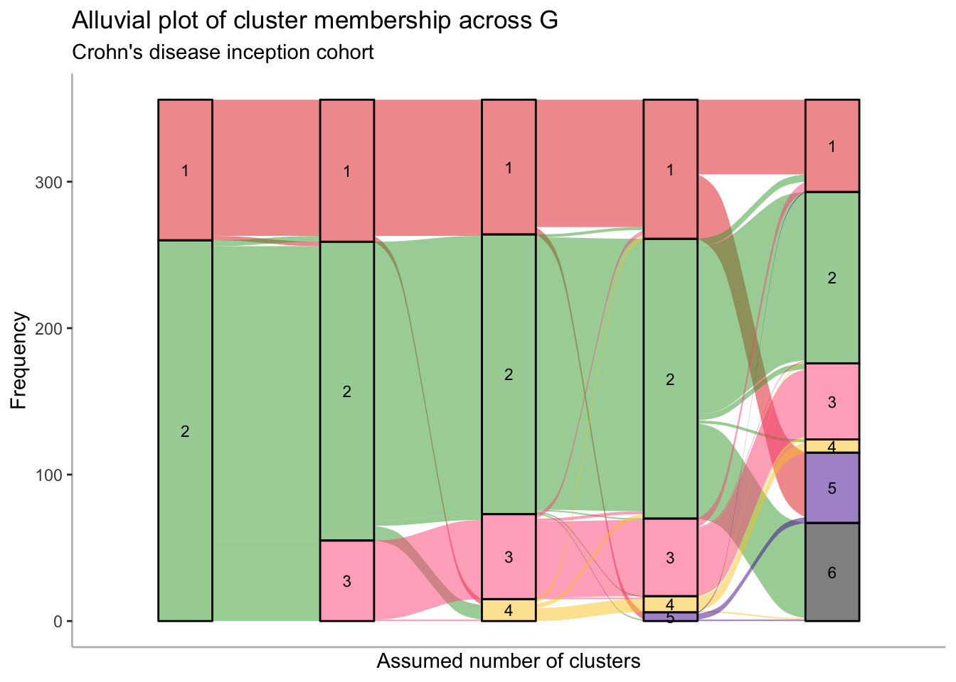
Considering all of the models above, AIC is most optimal for the G = 5 model and BIC is optimal for the G = 2 model. However, considering an alluvial plot (Figure 4) suggests neither G = 2 nor G = 5 are suitable models. The G = 2 model clearly has additional well defined cluster not properly represented by just two clusters, whilst the G=5 model results in an incredibly small new cluster. As such, G = 4 may be a more suitable alternative.

Cluster discrimination

Alluvial plots

Code

re_label <- function(old.G, new.G, alluvial.df){
  
  new.order <- rep(new.G, new.G)
  old.clusters <- subset(alluvial.df, G == old.G)
  new.clusters <- subset(alluvial.df, G == new.G)

  for (g in old.G:1) {
    ids <- subset(old.clusters, class == g)$id
    for (new.g in 1:new.G) {
      new.clusters.g <- subset(new.clusters, new.g == class)
      if (nrow(subset(new.clusters.g, id %in% ids)) > 0.5 * length(ids)) {
        new.order[new.g] <- g 
      }
    }
  }
  
  alluvial.df[alluvial.df[, "G"] == new.G, "class"] <-
    plyr::mapvalues(alluvial.df[alluvial.df[, "G"] == new.G, "class"],
                    from = seq(1, new.G),
                    new.order)
  return(alluvial.df)
}

# convert to alluvial format
alluvial.df <-cbind(groups.2$pprob[, 1:2], G = 2)
alluvial.df <-rbind(alluvial.df, cbind(groups.3$pprob[, 1:2], G = 3))
alluvial.df <-rbind(alluvial.df, cbind(groups.4$pprob[, 1:2], G = 4))
alluvial.df <-rbind(alluvial.df, cbind(groups.5$pprob[, 1:2], G = 5))
alluvial.df <-rbind(alluvial.df, cbind(groups.6$pprob[, 1:2], G = 6))
alluvial.df$id <- as.character(alluvial.df$id)
alluvial.df$class <- as.factor(alluvial.df$class) 

# eliminate label switching
alluvial.df <- re_label(2, 3, alluvial.df)
alluvial.df <- re_label(3, 4, alluvial.df)
alluvial.df <- re_label(4, 5, alluvial.df)
alluvial.df <- re_label(5, 6, alluvial.df)

p <- ggplot(alluvial.df,
            aes(x = G,
            stratum = class,
            alluvium = id,
            fill = class,
            label = class)) + 
  scale_x_discrete(expand = c(.1, .1)) +
  geom_flow()  +
  geom_stratum(alpha = 0.5) +
  geom_text(stat = "stratum", size = 3) +
  theme_classic() +
  theme(axis.line = element_line(colour = "gray")) +
  theme(legend.position = "none") +
  ggtitle("Alluvial plot of cluster membership across G",
          "Crohn's disease inception cohort") +
  scale_fill_manual(values = c("#e3281f",
                               "#3aa534",
                               "#ff5885",
                               "#fbc926",
                               "#511e9d",
                               "black")) +
  xlab("Assumed number of clusters") + 
  ylab("Frequency")
print(p)

p <- p + ggtitle("", "")
ggsave("paper/alluvial.png", p, width = 8, height = 4.5, units = "in")
ggsave("paper/alluvial.pdf", p, width = 8, height = 4.5, units = "in")

Figure 4: Alluvial plot demonstrating how cluster membership changes as the assumed number of clusters increase. The height of each band indicates the size of each cluster.

Posterior classifications

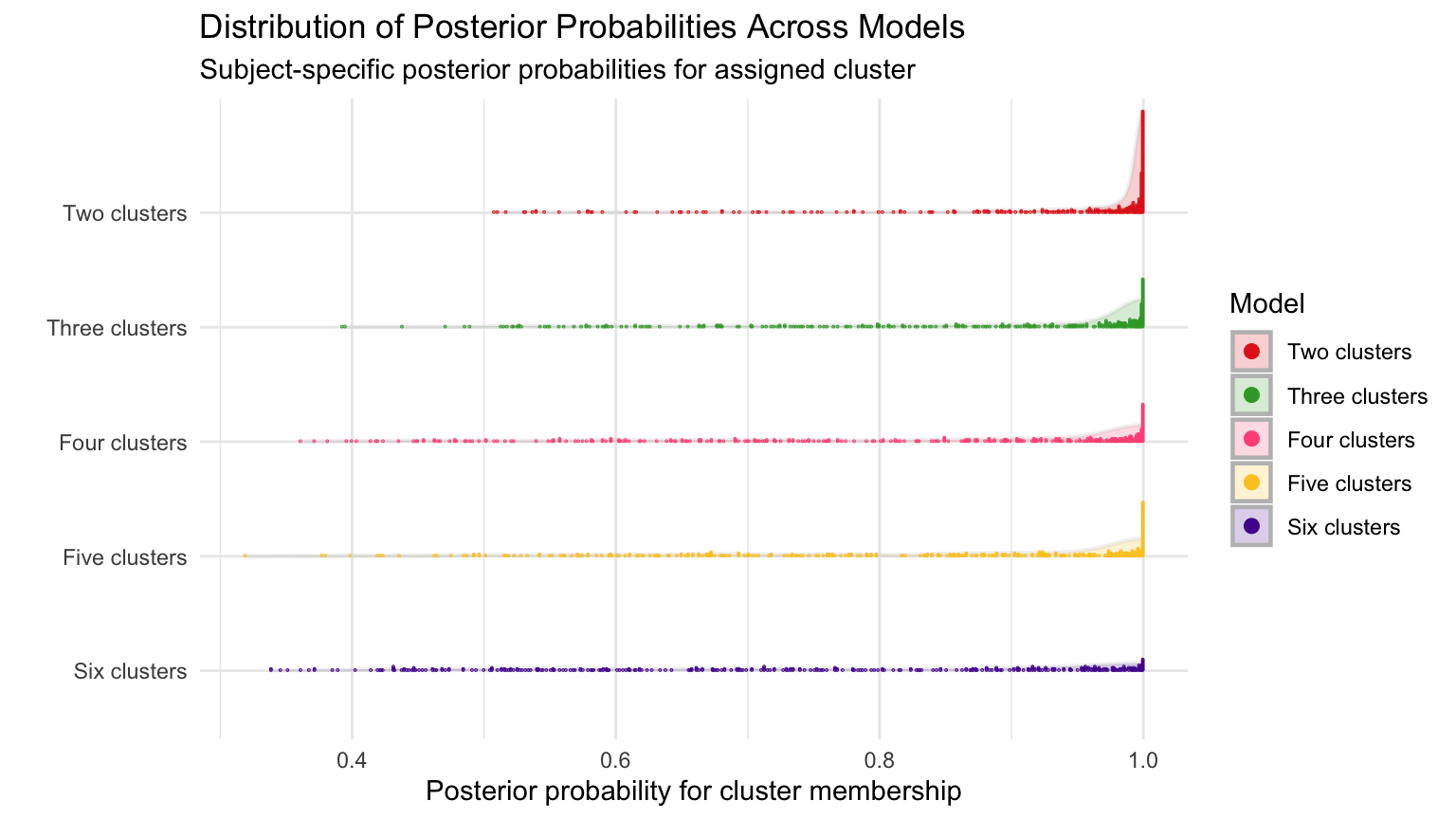
An alternative to co-clustering when considering cluster discrimination is to consider posterior classification possibilities. From the below data, we can see how these posterior probabilities change as the number of assumed clusters increase

Code

postprob(cubicbf.fits[[2]])

 
Posterior classification: 
  class1 class2
N  96.00 260.00
%  26.97  73.03
 
Posterior classification table: 
     --> mean of posterior probabilities in each class 
        prob1  prob2
class1 0.8747 0.1253
class2 0.0506 0.9494
 
Posterior probabilities above a threshold (%): 
         class1 class2
prob>0.7  80.21  95.38
prob>0.8  70.83  92.31
prob>0.9  62.50  83.08

Code

postprob(cubicbf.fits[[3]])

 
Posterior classification: 
  class1 class2 class3
N  97.00  204.0  55.00
%  27.25   57.3  15.45
 
Posterior classification table: 
     --> mean of posterior probabilities in each class 
        prob1  prob2  prob3
class1 0.8678 0.0789 0.0533
class2 0.0366 0.8925 0.0710
class3 0.0606 0.1298 0.8095
 
Posterior probabilities above a threshold (%): 
         class1 class2 class3
prob>0.7  80.41  88.24  70.91
prob>0.8  68.04  77.45  60.00
prob>0.9  57.73  65.20  43.64

Code

postprob(cubicbf.fits[[4]])

 
Posterior classification: 
  class1 class2 class3 class4
N  15.00  58.00  92.00 191.00
%   4.21  16.29  25.84  53.65
 
Posterior classification table: 
     --> mean of posterior probabilities in each class 
        prob1  prob2  prob3  prob4
class1 0.7105 0.0549 0.0944 0.1401
class2 0.0540 0.7997 0.0484 0.0978
class3 0.0707 0.0653 0.8191 0.0449
class4 0.0747 0.0618 0.0229 0.8406
 
Posterior probabilities above a threshold (%): 
         class1 class2 class3 class4
prob>0.7  53.33  65.52  71.74  78.01
prob>0.8  46.67  58.62  63.04  64.92
prob>0.9  13.33  39.66  51.09  53.93

Code

postprob(cubicbf.fits[[5]])

 
Posterior classification: 
  class1 class2 class3 class4 class5
N  95.00 191.00   6.00  11.00  53.00
%  26.69  53.65   1.69   3.09  14.89
 
Posterior classification table: 
     --> mean of posterior probabilities in each class 
        prob1  prob2  prob3  prob4  prob5
class1 0.8229 0.0664 0.0353 0.0336 0.0418
class2 0.0291 0.8529 0.0048 0.0645 0.0488
class3 0.1424 0.0132 0.8431 0.0012 0.0001
class4 0.0209 0.1351 0.0000 0.7499 0.0940
class5 0.0663 0.0763 0.0001 0.0572 0.8001
 
Posterior probabilities above a threshold (%): 
         class1 class2 class3 class4 class5
prob>0.7  74.74  76.96  66.67  63.64  67.92
prob>0.8  60.00  66.49  66.67  45.45  54.72
prob>0.9  47.37  53.40  50.00  36.36  39.62

Code

postprob(cubicbf.fits[[6]])

 
Posterior classification: 
  class1 class2 class3 class4 class5 class6
N  48.00   63.0  52.00 117.00  67.00   9.00
%  13.48   17.7  14.61  32.87  18.82   2.53
 
Posterior classification table: 
     --> mean of posterior probabilities in each class 
        prob1  prob2  prob3  prob4  prob5  prob6
class1 0.8604 0.1241 0.0070 0.0001 0.0043 0.0042
class2 0.0798 0.7354 0.0588 0.0092 0.1022 0.0147
class3 0.0016 0.0447 0.7671 0.0471 0.0893 0.0501
class4 0.0003 0.0067 0.0439 0.7737 0.1381 0.0373
class5 0.0022 0.1143 0.0554 0.1256 0.6373 0.0651
class6 0.0004 0.0169 0.0223 0.0490 0.1295 0.7818
 
Posterior probabilities above a threshold (%): 
         class1 class2 class3 class4 class5 class6
prob>0.7  87.50  57.14  65.38  60.68  32.84  77.78
prob>0.8  66.67  42.86  53.85  52.99  17.91  55.56
prob>0.9  58.33  26.98  36.54  41.03  13.43  44.44

Code

pprobs.2 <- c()
pprobs.3 <- c()
pprobs.4 <- c()
pprobs.5 <- c()
pprobs.6 <- c()
for (i in 1:nrow(cubicbf.fits[[1]]$pprob)){
  class.2 <- groups.2$pprob[i, 2]
  pprobs.2 <- c(pprobs.2, groups.2$pprob[i, class.2 + 2 ])
  class.3 <- groups.3$pprob[i, 2]
  pprobs.3 <- c(pprobs.3, groups.3$pprob[i, class.3 + 2 ])
  class.4 <- groups.4$pprob[i, 2]
  pprobs.4 <- c(pprobs.4, groups.4$pprob[i, class.4 + 2 ])
  class.5 <- groups.5$pprob[i, 2]
  pprobs.5 <- c(pprobs.5, groups.5$pprob[i, class.5 + 2 ])
  class.6 <- groups.6$pprob[i, 2]
  pprobs.6 <- c(pprobs.6, groups.6$pprob[i, class.6 + 2 ])
}
pprobs.2 <- tibble(prob = pprobs.2)
pprobs.3 <- tibble(prob = pprobs.3)
pprobs.4 <- tibble(prob = pprobs.4)
pprobs.5 <- tibble(prob = pprobs.5)
pprobs.6 <- tibble(prob = pprobs.6)

pprobs.2$Model <- as.factor(rep("Two clusters", nrow(pprobs.2)))
pprobs.3$Model <- as.factor(rep("Three clusters", nrow(pprobs.3)))
pprobs.4$Model <- as.factor(rep("Four clusters", nrow(pprobs.4)))
pprobs.5$Model <- as.factor(rep("Five clusters", nrow(pprobs.5)))
pprobs.6$Model <- as.factor(rep("Six clusters", nrow(pprobs.6)))
pprobs <- rbind(pprobs.2, pprobs.3, pprobs.4, pprobs.5, pprobs.6)

p <- pprobs %>%
  ggplot(aes(x = prob, y = Model)) +
  #geom_histogram(bins = 40, fill = NA, position="identity")
  stat_slab(aes(fill = Model),color = "gray",
                    size = 0.8,
                    alpha = 0.2) +
  geom_dots(aes(fill = Model, color = Model), dotsize = 1) +
  xlab("Posterior probability for cluster membership") +
  ylab("") + 
  ggtitle("Distribution of Posterior Probabilities Across Models",
          "Subject-specific posterior probabilities for assigned cluster") +
  theme_minimal() + 
  scale_color_manual(values = c("#e3281f",
                                "#3aa534",
                                "#ff5885",
                                "#fbc926",
                                "#511e9d")
                     ) +
  scale_fill_manual(values = c("#e3281f",
                               "#3aa534",
                               "#ff5885",
                               "#fbc926",
                               "#511e9d")
                    ) +
  scale_y_discrete(limits = rev)
print(p)

Code

ggsave("plots/Distributions.png", p, width = 8.5, height = 4.5, units = "in")
ggsave("plots/Distributions.pdf", p, width = 8.5, height = 4.5, units = "in")

Residual plots

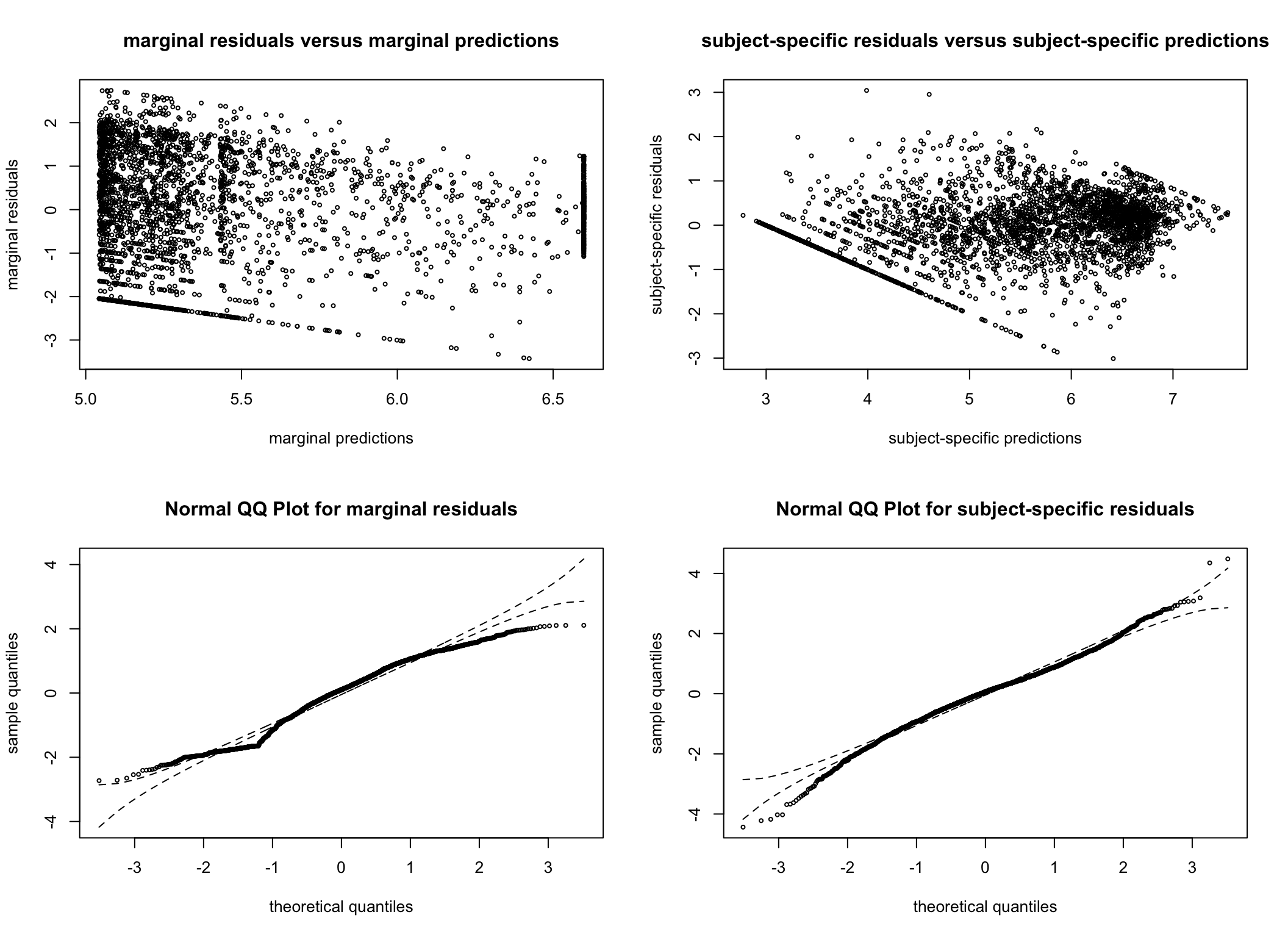
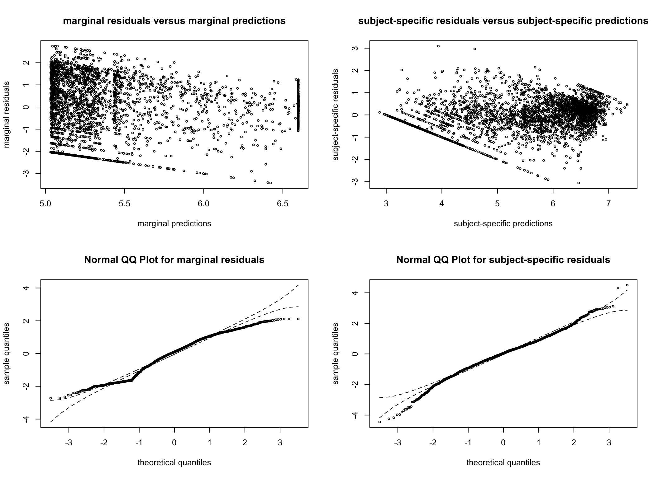
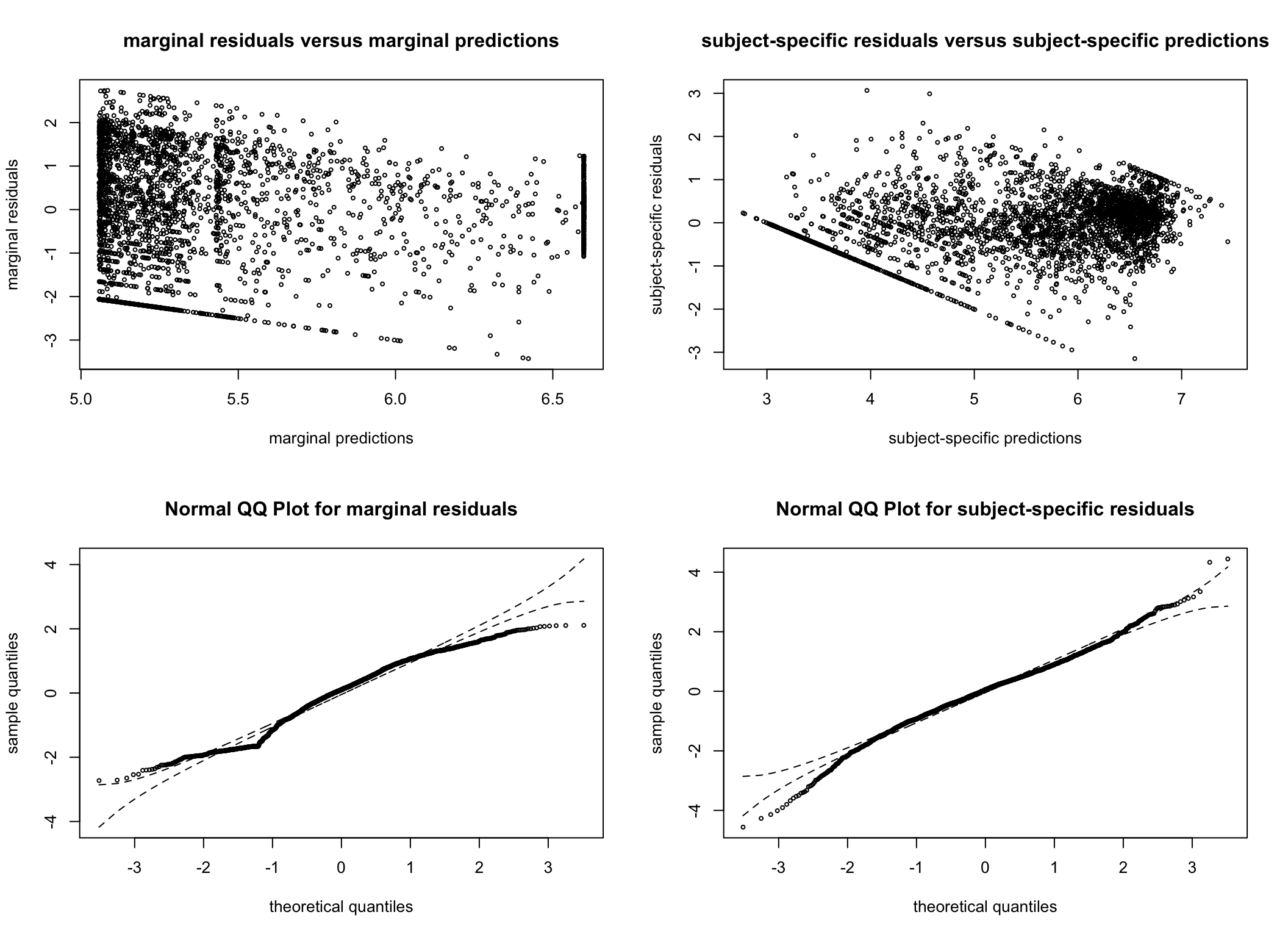
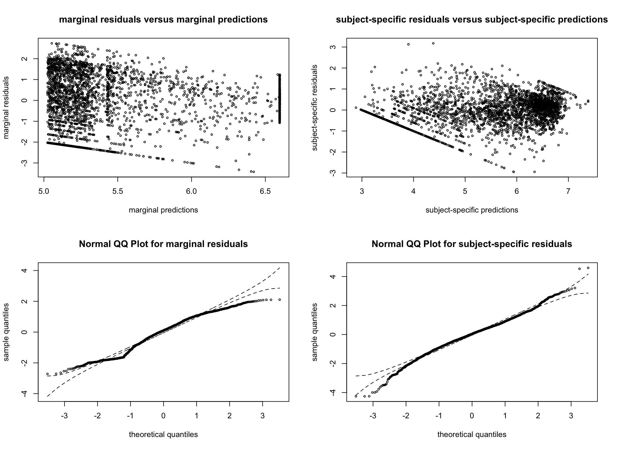
To ensure model assumptions are not violated, residual plots are also consulted. The residual plots are very similar across all models considered and are reassuring. As we later decide on the G = 4 model (see the Spaghetti plots per cluster section), we have generated additional plots examining the normality of the residuals for this model.

Code

plot(cubicbf.fits[[1]], shades = TRUE)

Code

plot(cubicbf.fits[[2]], shades = TRUE)

Code

plot(cubicbf.fits[[3]], shades = TRUE)

Code

plot(cubicbf.fits[[4]], shades = TRUE)

Code

p1 <- data.frame(residuals = resid(cubicbf.fits[[4]])) %>%
  ggplot(aes(x = residuals)) +
  geom_histogram(aes(y = ..density..),
                 fill = "#D8829D",
                 color = "#AF6A80",
                 bins = 30) +
  geom_density(color = "#023777", size = 1.2) +
  theme_classic() +
  theme(axis.line = element_line(colour = "gray")) +
  ylab("Density") +
  xlab("Residuals") +
  ggtitle("A")

Warning: Using `size` aesthetic for lines was deprecated in ggplot2 3.4.0.
ℹ Please use `linewidth` instead.

Code

p2 <- data.frame(residuals = resid(cubicbf.fits[[4]])) %>%
  ggplot(aes(sample = residuals)) +
    stat_qq_band() +
    stat_qq_line(color = "#D8829D") +
    stat_qq_point(color = "#023777")  +
    theme_classic() +
    theme(axis.line = element_line(colour = "gray")) + 
    ylab("Theoretical Quantiles") +
    xlab("Sample Quantiles") +
  ggtitle("B")
ggsave("paper/Residual-plot.pdf",
       plot = p1 / p2,
       width = 8,
       height = 8,
       units = "in")

Warning: The dot-dot notation (`..density..`) was deprecated in ggplot2 3.4.0.
ℹ Please use `after_stat(density)` instead.

Code

print(p1 / p2)

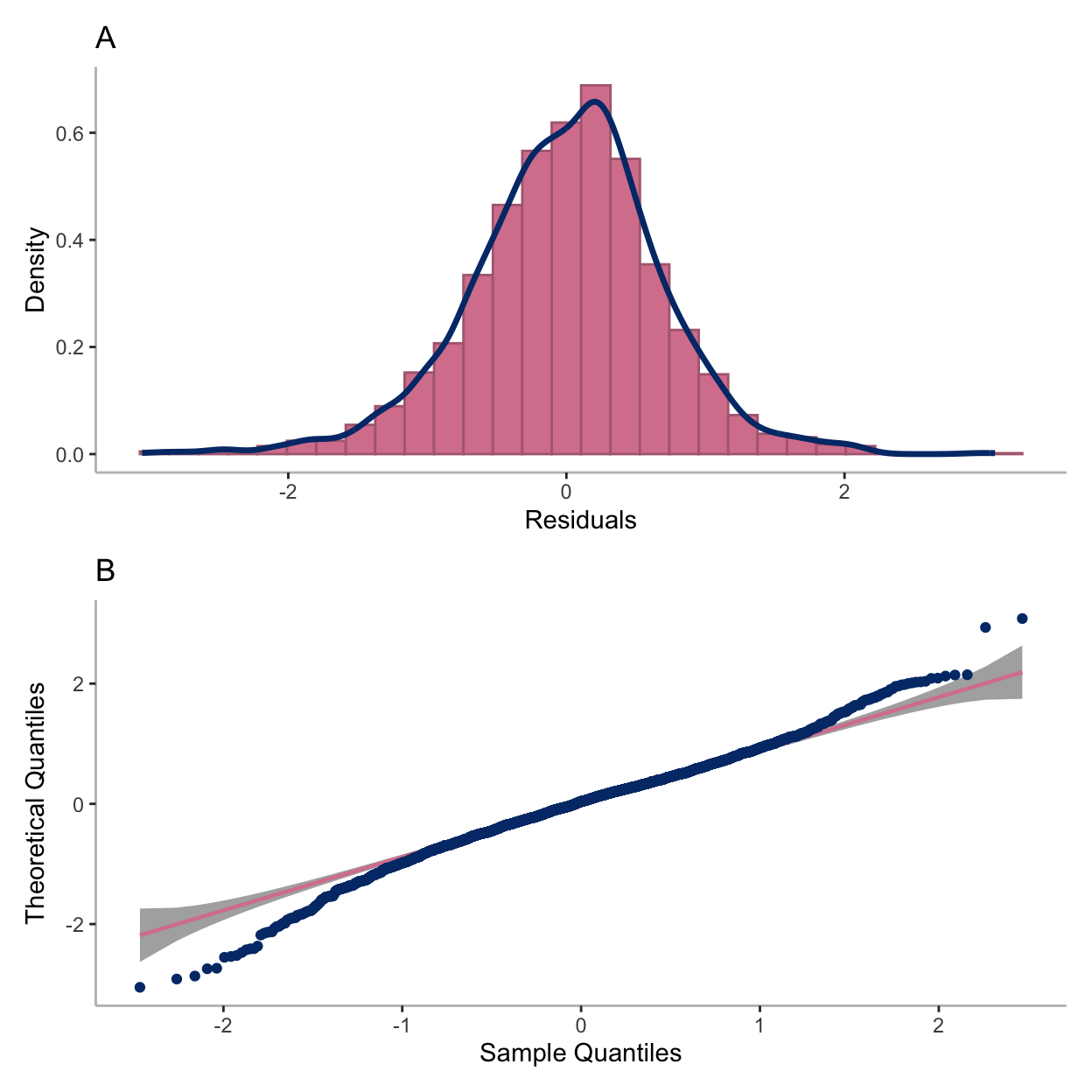
Figure 5: (A) Density plot of residuals for the four-cluster model. (B) Quantile-quantile plot of residuals for the four-cluster model.

Code

dict <- cubicbf.fits[[4]]$pprob[, c("id", "class")]
dict$class <- plyr::mapvalues(dict$class,
                              from = c(1, 2, 3, 4),
                              to = c(4, 3, 1, 2))
temp <- merge(cubicbf.fits[[4]]$pred, dict, by = "id")
par(mfrow = c(2,2))
labels <- c("A", "B", "C", "D")
p <- list()

for (i in 1:4) {
  p[[i]] <- subset(temp, class == i) %>%
    ggplot(aes(sample = resid_ss)) +
    stat_qq_band() +
    stat_qq_line(color = "#D8829D") +
    stat_qq_point(color = "#023777")  +
    theme_classic() +
    theme(axis.line = element_line(colour = "gray")) + 
    ylab("Theoretical Quantiles") +
    xlab("Sample Quantiles") +
  ggtitle(labels[i])
}
ggsave("paper/cluster-resids.pdf",
       (p[[1]] + p[[2]]) / (p[[3]] + p[[4]]),
       width = 8,
       height = 8,
       units = "in")
print((p[[1]] + p[[2]]) / (p[[3]] + p[[4]]))

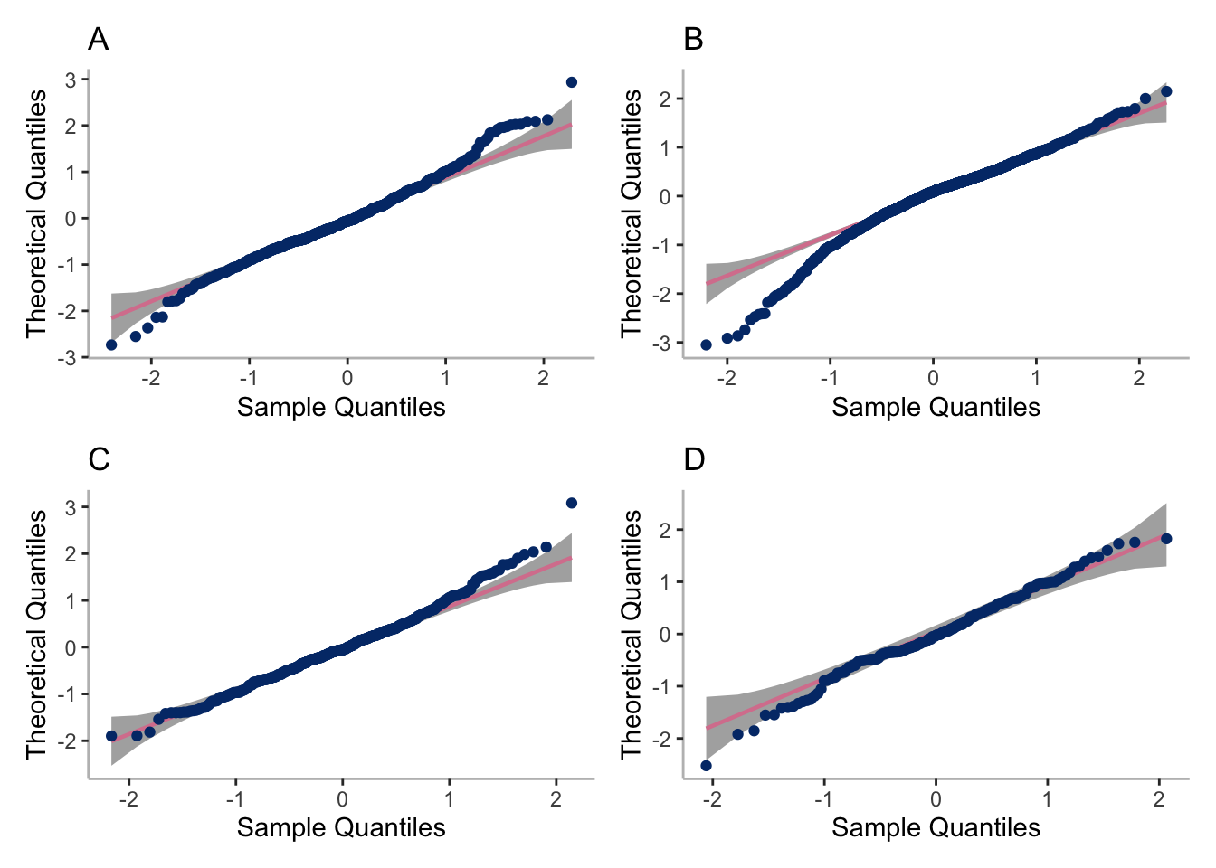
Figure 6: Quantile-quantile plots of residuals for the four-cluster latent class mixed model stratified by (A) cluster 1; (B) cluster 2; (C) cluster 3; and (D) cluster 4.

Code

plot(cubicbf.fits[[5]], shades = TRUE)

Code

plot(cubicbf.fits[[6]], shades = TRUE)

Spaghetti plots per cluster

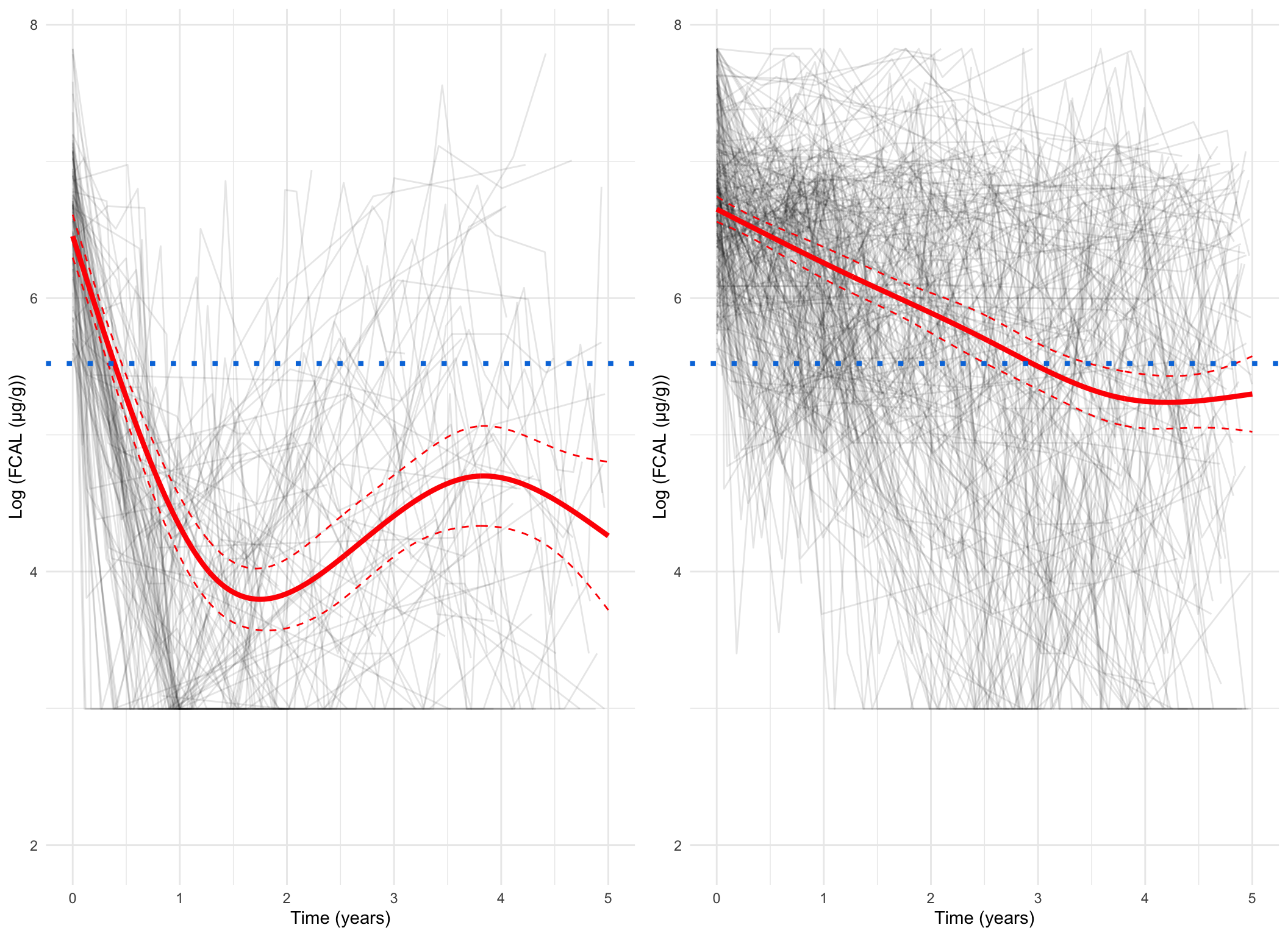
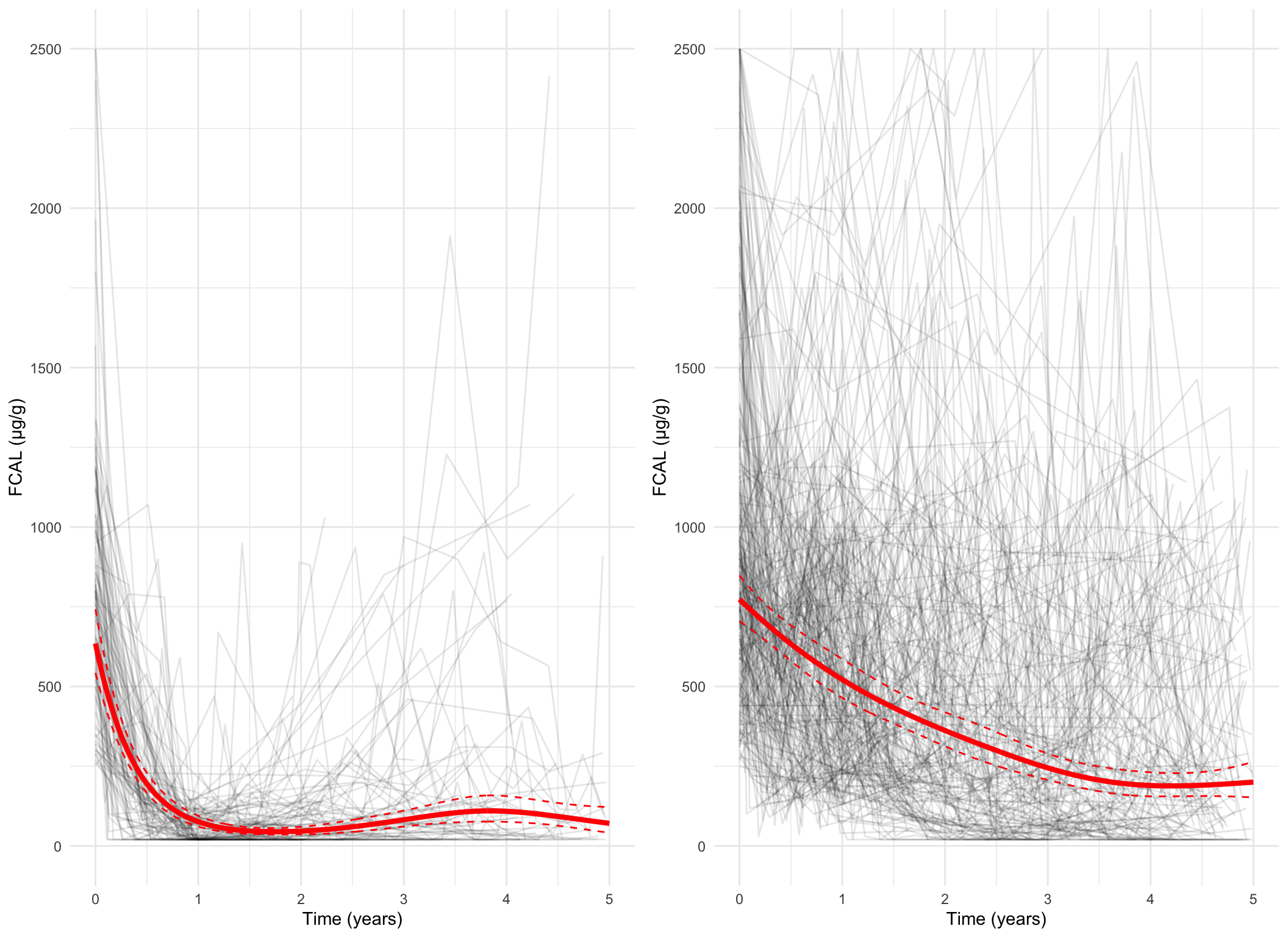
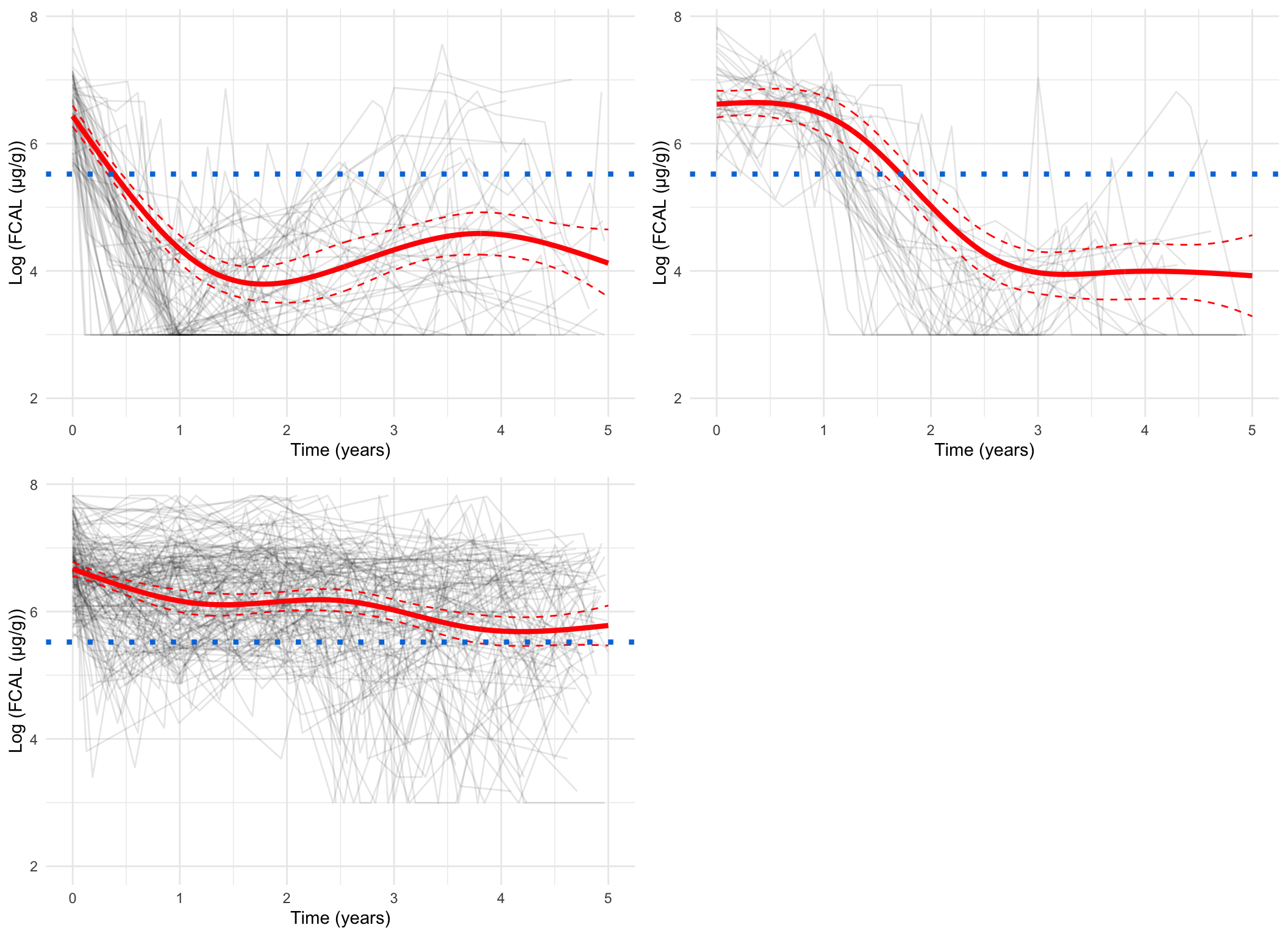
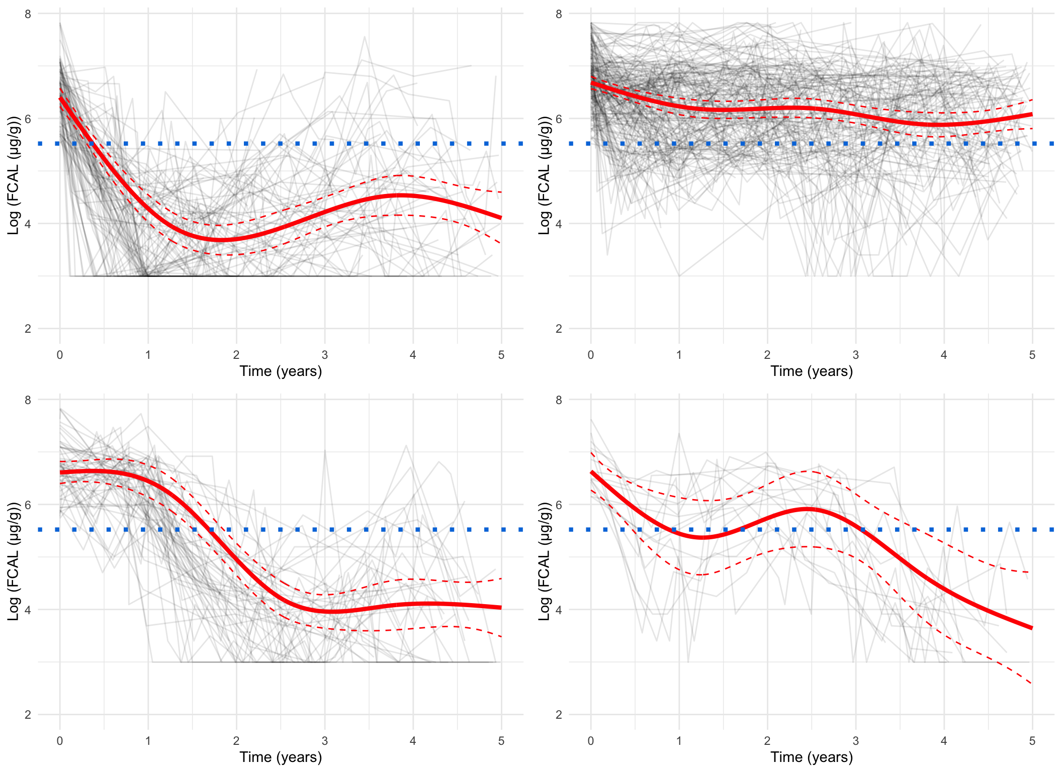
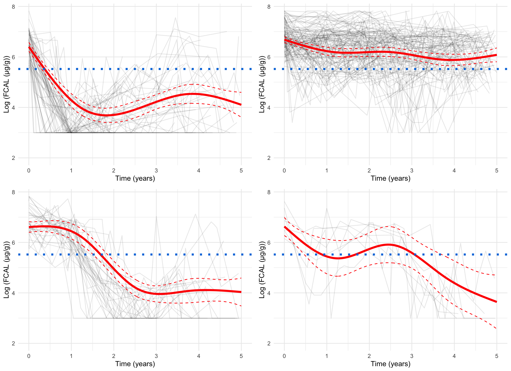
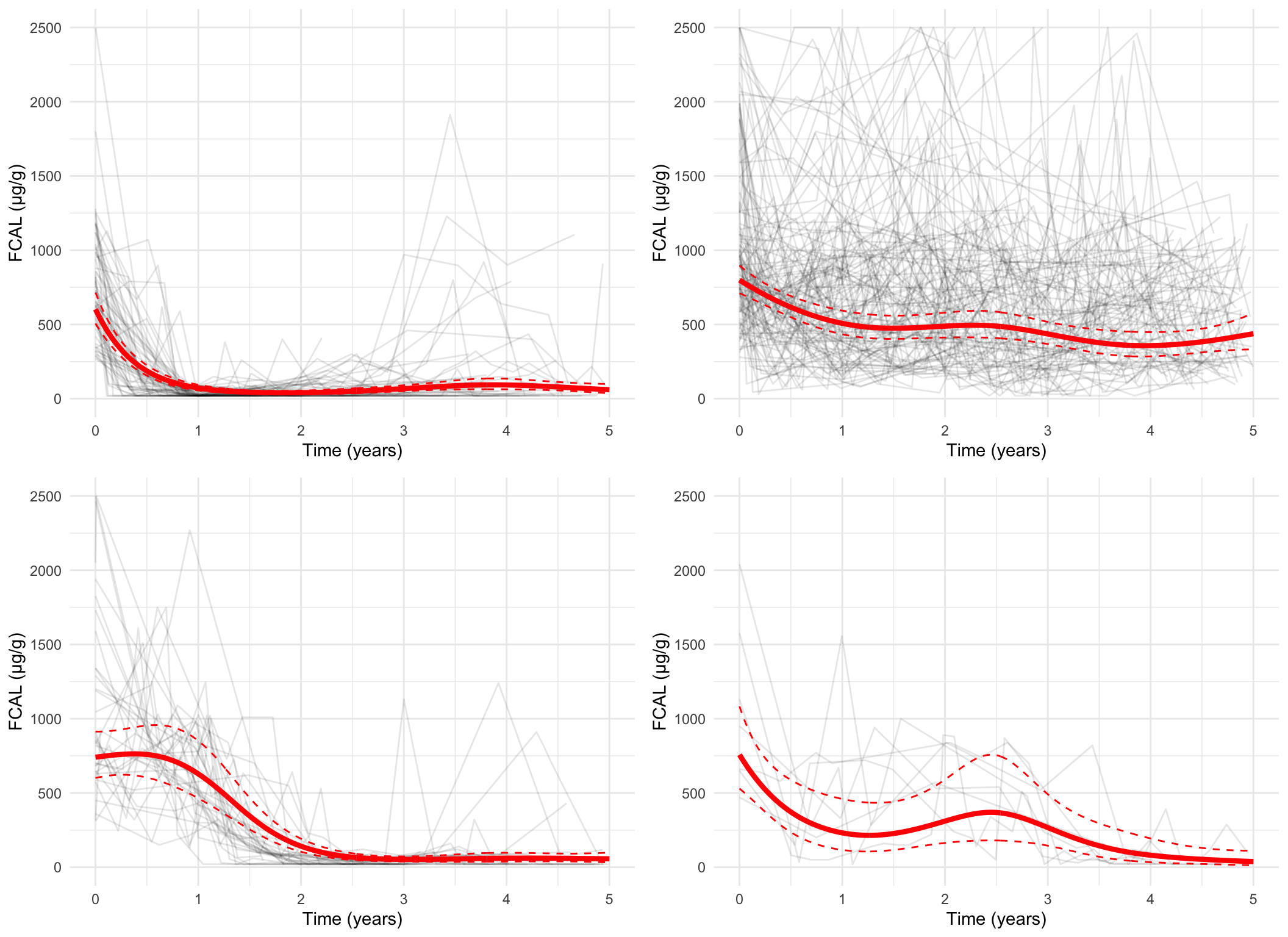
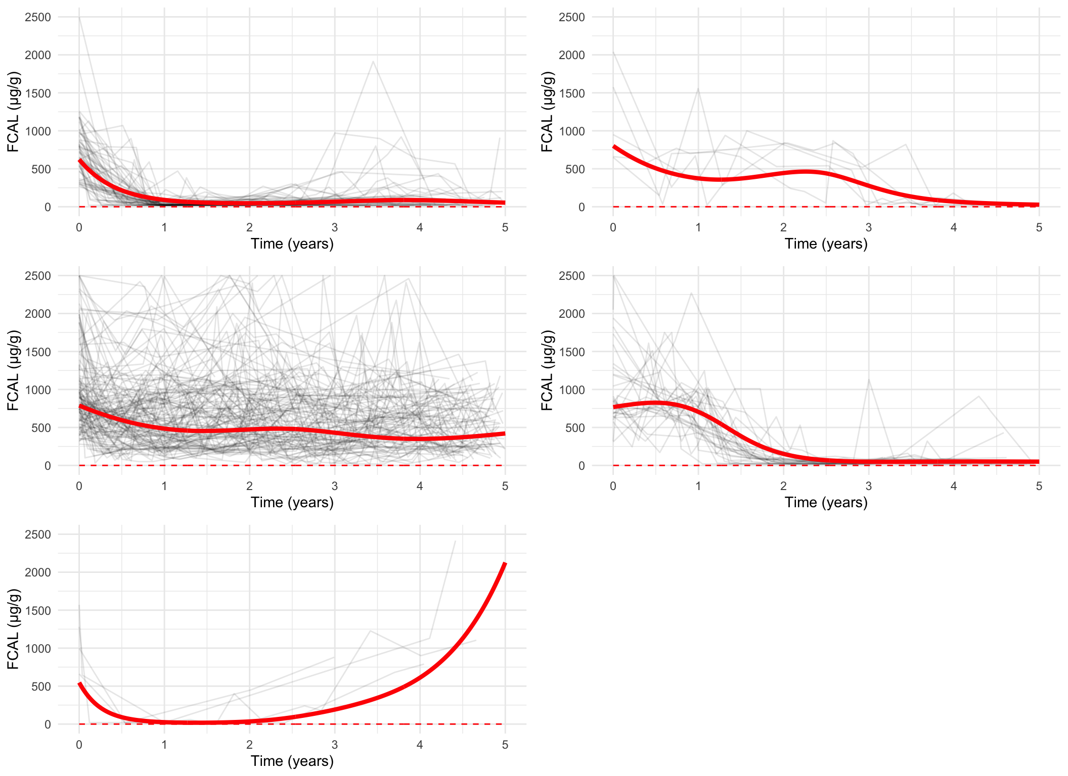
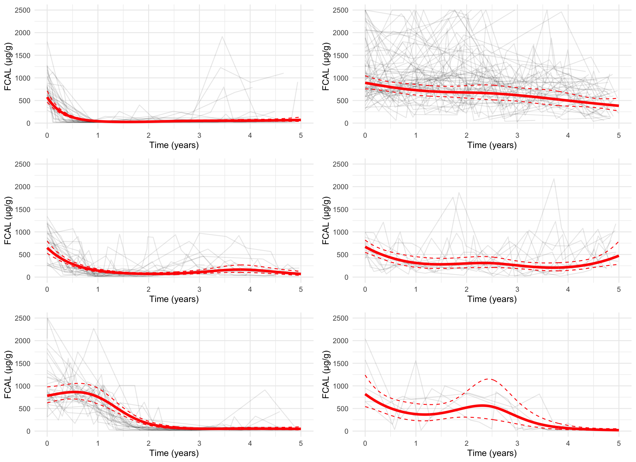
Plotting the mean cluster trajectories alongside spaghetti plots of all subject trajectories provides evidence for the G = 4 model being the most appropriate.

Log-scale, all subjects

Code

spaghetti_plot(FCcumulative, cubicbf.fits, G = 2, log = TRUE, sizes = TRUE)

There are 96 subjects in cluster 1.

There are 260 subjects in cluster 2.

Measurement-scale, all subjects

Code

spaghetti_plot(FCcumulative, cubicbf.fits, G = 2, log = FALSE)

Log-scale, pprob > 0.8 only

Code

spaghetti_plot(FCcumulative,
               cubicbf.fits,
               G = 2,
               log = TRUE,
               pprob.cutoff = 0.8)

Measurement-scale, pprob > 0.8 only

Code

spaghetti_plot(FCcumulative,
               cubicbf.fits,
               G = 2,
               log = FALSE,
               pprob.cutoff = 0.8)

Log-scale, all subjects

Code

#| fig-width: 11
#| fig.height: 8
spaghetti_plot(FCcumulative,
               cubicbf.fits,
               G = 3,
               log = TRUE,
               mapping = c(1,3,2),
               sizes = TRUE)

There are 97 subjects in cluster 1.

There are 204 subjects in cluster 3.

There are 55 subjects in cluster 2.

Measurement-scale, all subjects

Code

spaghetti_plot(FCcumulative, cubicbf.fits, G = 3, log = FALSE)

Log-scale, pprob > 0.8 only

Code

spaghetti_plot(FCcumulative,
               cubicbf.fits,
               G = 3,
               log = TRUE,
               pprob.cutoff = 0.8)

Measurement-scale, pprob > 0.8 only

Code

spaghetti_plot(FCcumulative,
               cubicbf.fits,
               G = 3,
               log = FALSE,
               pprob.cutoff = 0.8)

Class membership has been relabelled to ensure consistency with the alluvial plot

Log-scale, all subjects

Code

spaghetti_plot(FCcumulative,
               cubicbf.fits,
               G = 4,
               log = TRUE,
               mapping = c(3,2,4,1),
               sizes = TRUE)

There are 191 subjects in cluster 3.

There are 58 subjects in cluster 2.

There are 15 subjects in cluster 4.

There are 92 subjects in cluster 1.

Measurement-scale, all subjects

Code

spaghetti_plot(FCcumulative,
               cubicbf.fits,
               G = 4,
               log = FALSE,
               mapping = c(3, 2, 4, 1))

Log-scale, pprob > 0.8 only

Code

spaghetti_plot(FCcumulative,
               cubicbf.fits,
               G = 4,
               log = TRUE,
               pprob.cutoff = 0.8,
               mapping = c(3, 2, 4, 1))

Measurement-scale, pprob > 0.8 only

Code

spaghetti_plot(FCcumulative,
               cubicbf.fits,
               G = 4,
               log = FALSE,
               pprob.cutoff = 0.8,
               mapping = c(3, 2, 4, 1))

Log-scale, all subjects

Code

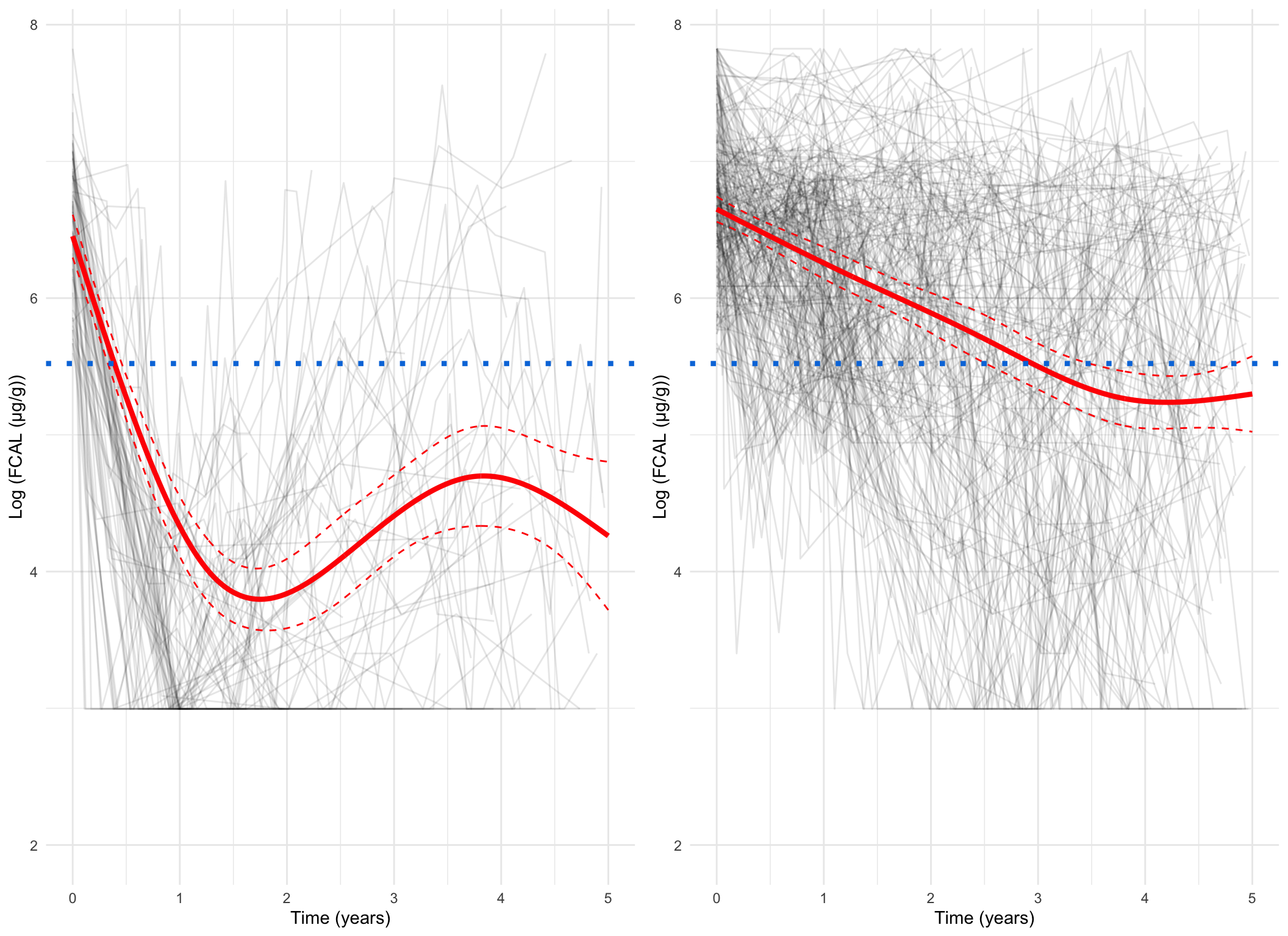
spaghetti_plot(FCcumulative, cubicbf.fits, G = 5, log = TRUE, sizes = TRUE)

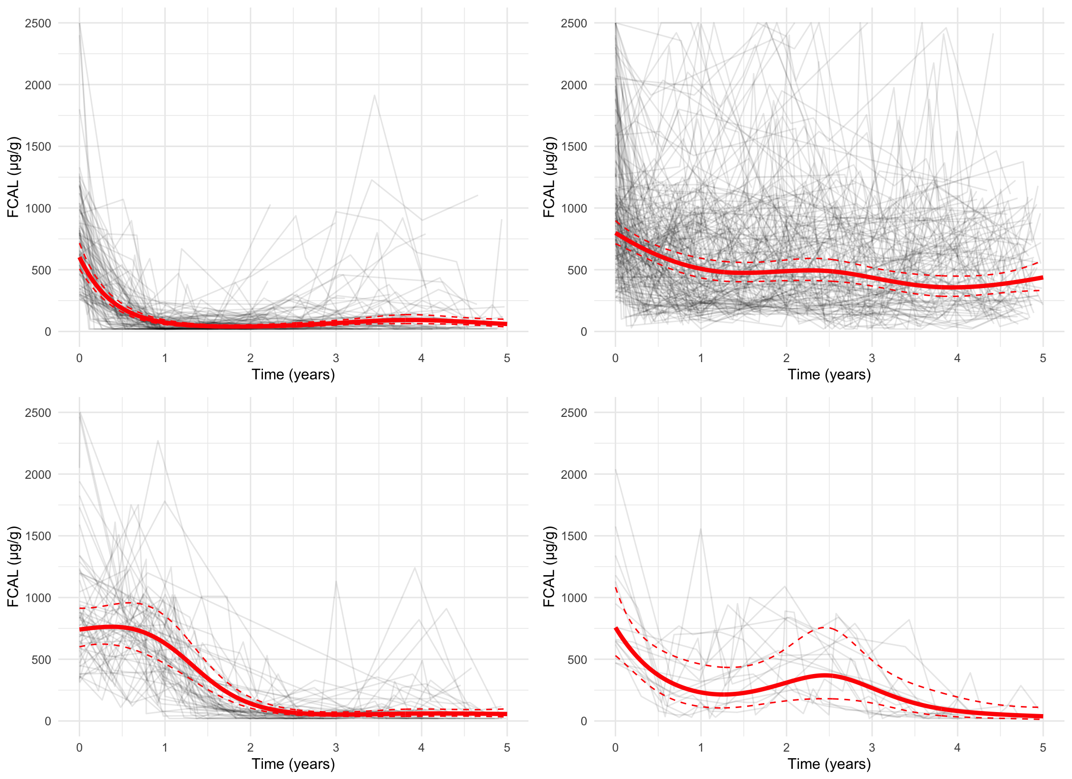
Measurement-scale, all subjects

Code

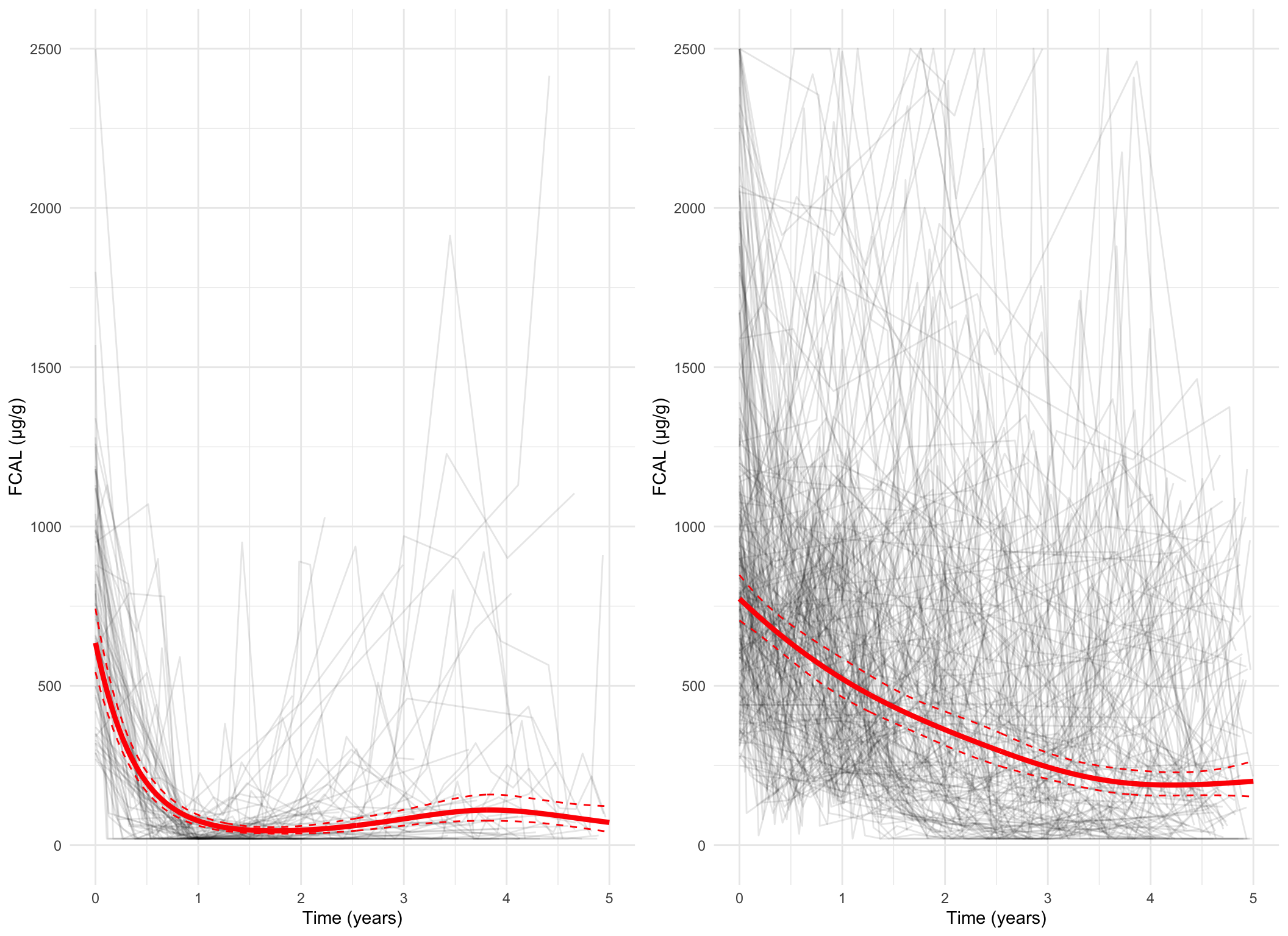
spaghetti_plot(FCcumulative, cubicbf.fits, G = 5, log = FALSE)

Log-scale, pprob > 0.8 only

Code

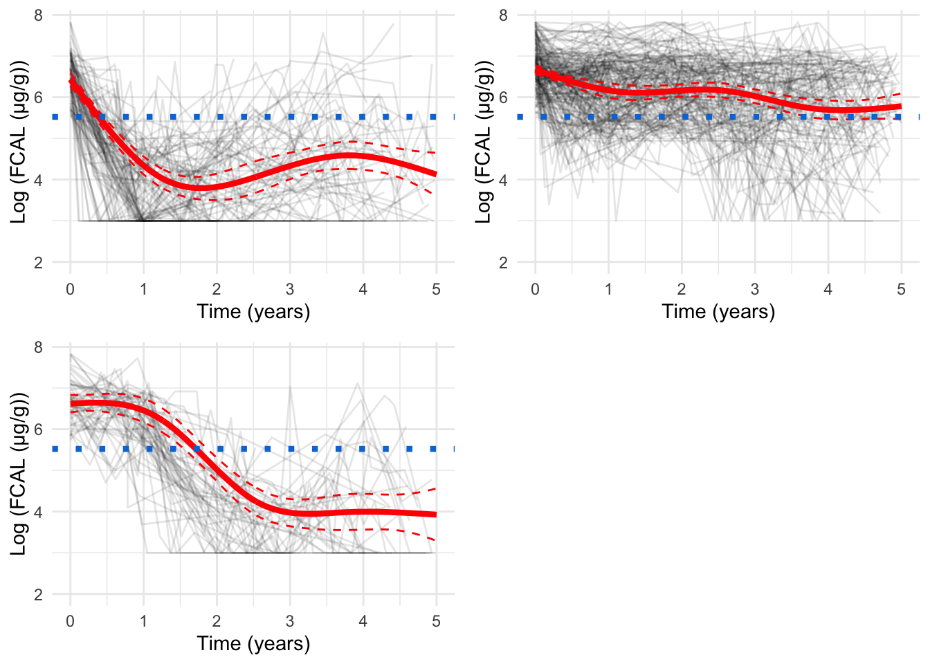
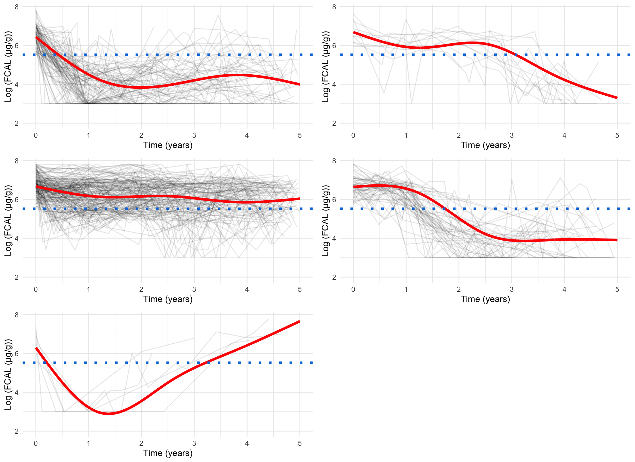
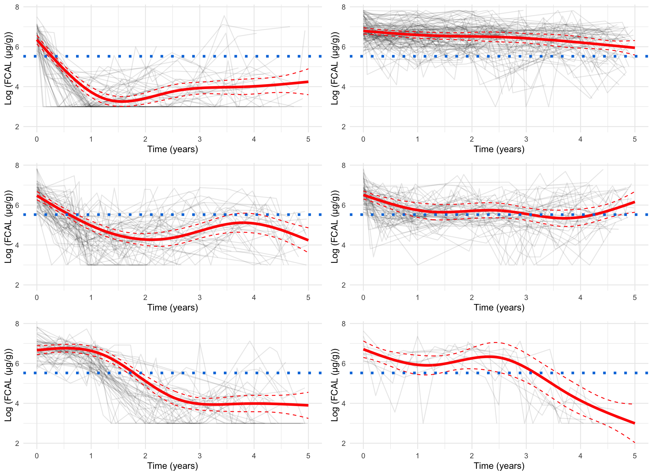
spaghetti_plot(FCcumulative,
               cubicbf.fits,
               G = 5,
               log = TRUE,
               pprob.cutoff = 0.8)

Measurement-scale, pprob > 0.8 only

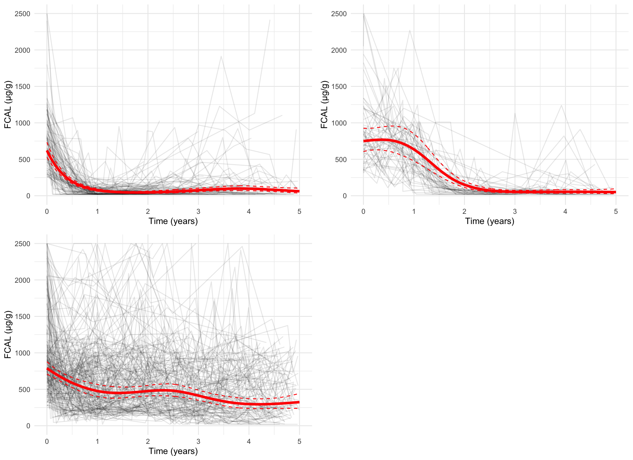
Code

spaghetti_plot(FCcumulative,
               cubicbf.fits,
               G = 5,
               log = FALSE,
               pprob.cutoff = 0.8)

Log-scale, all subjects

Code

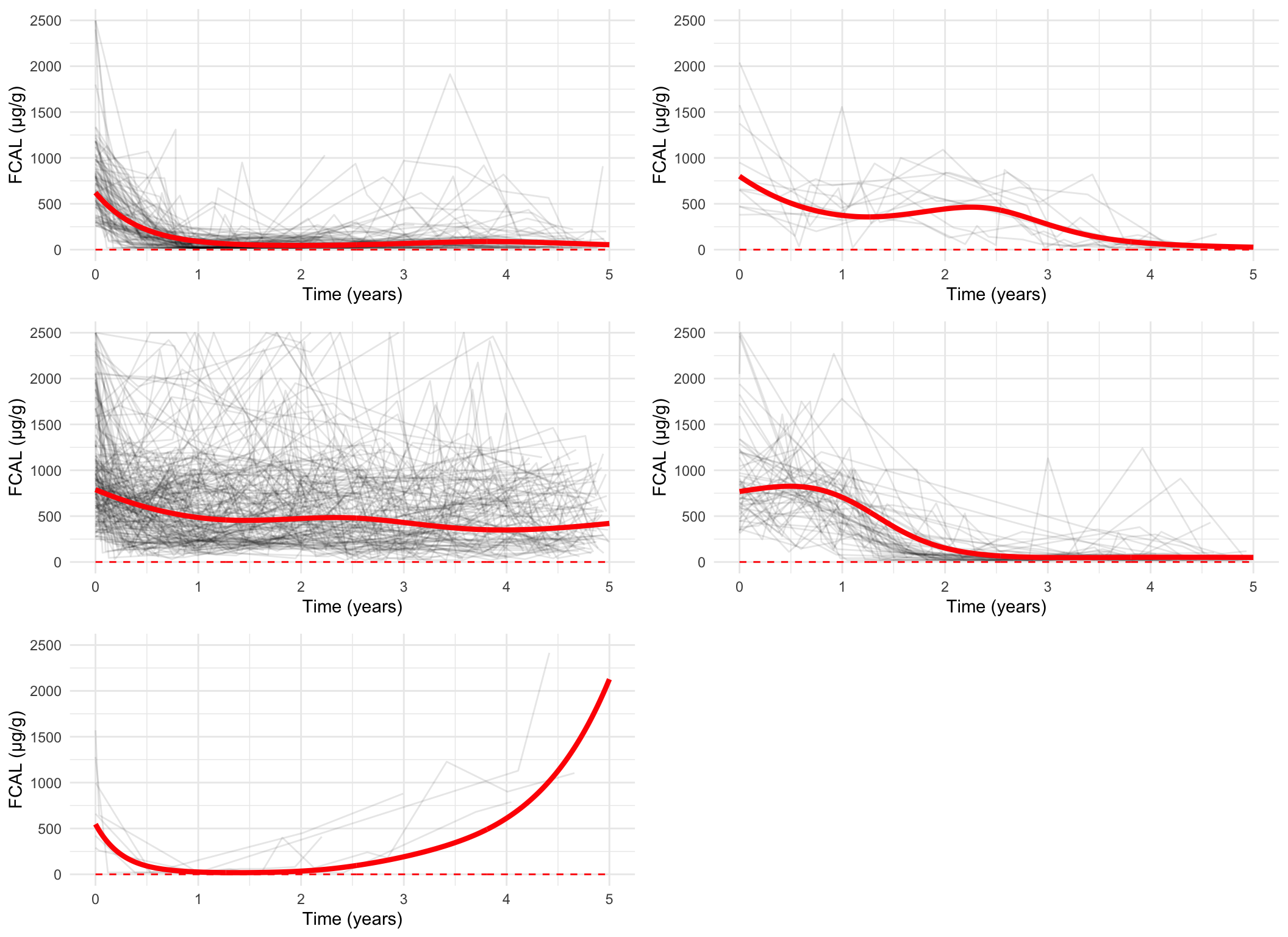
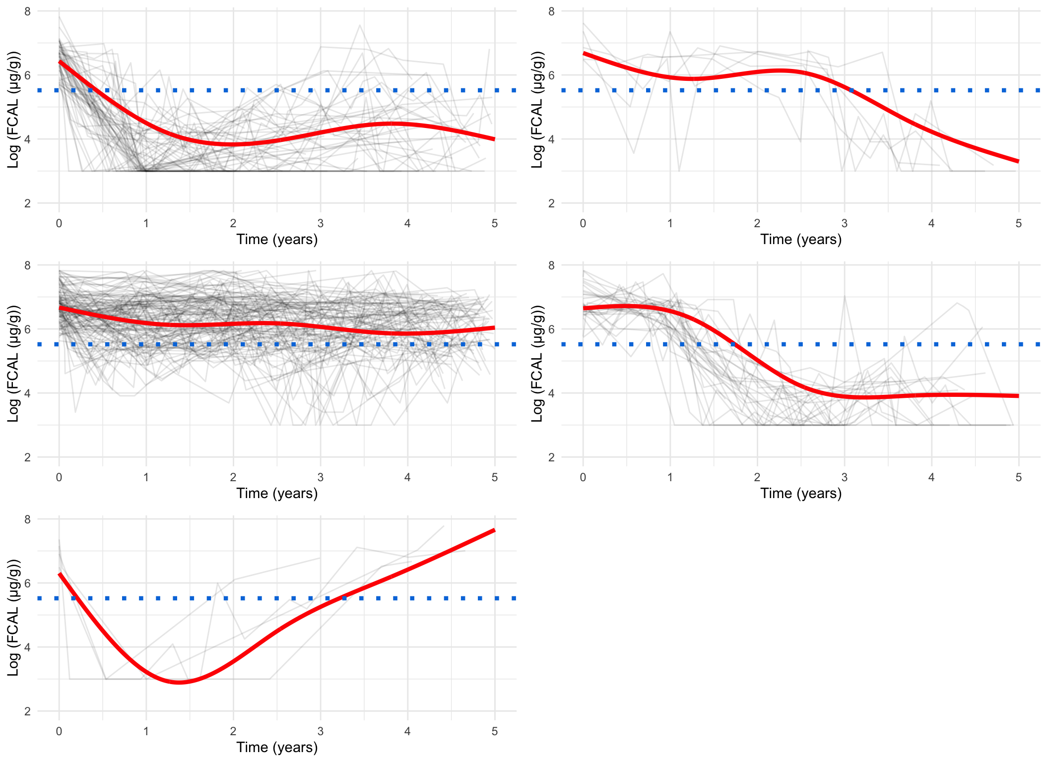
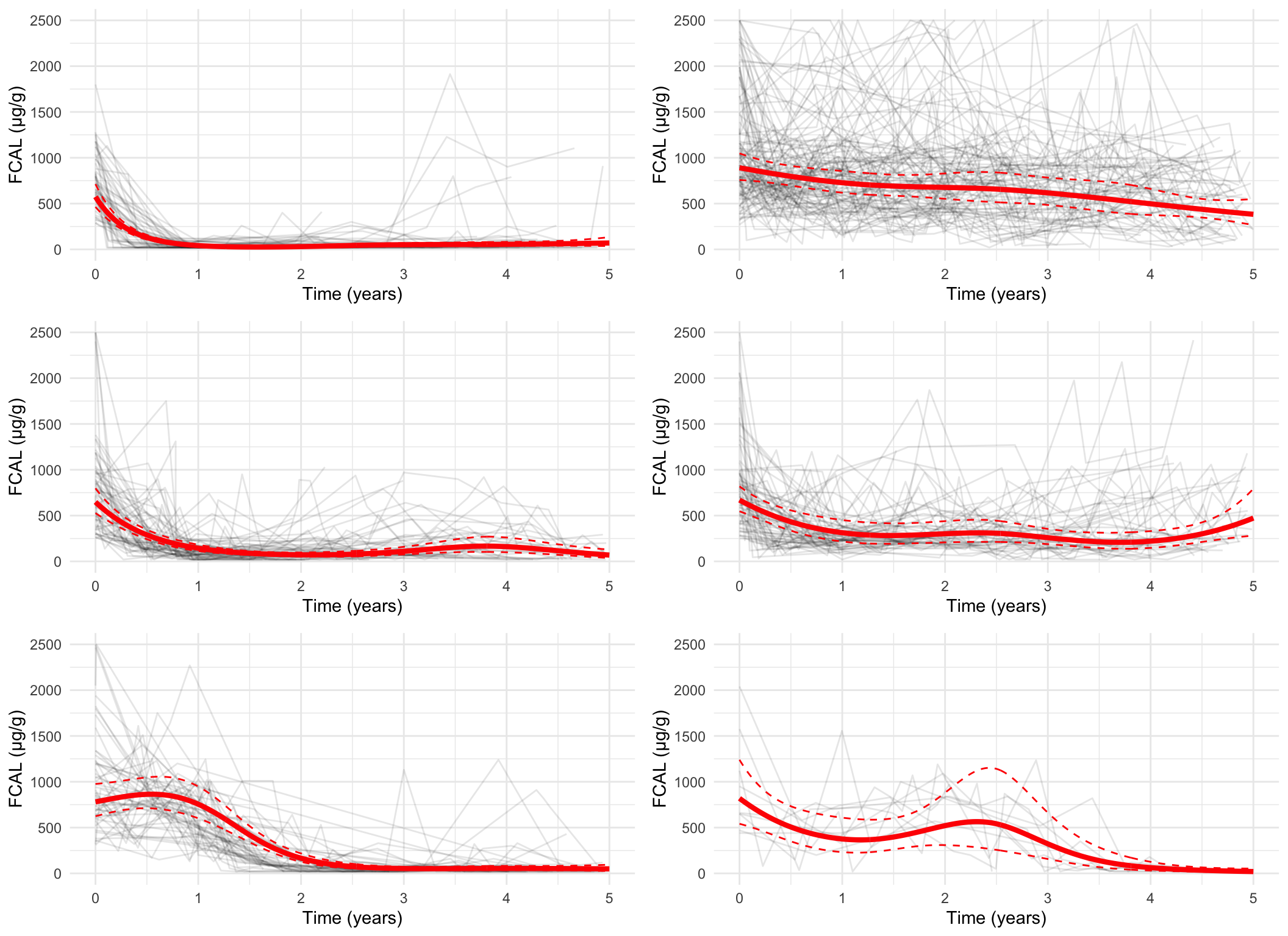
spaghetti_plot(FCcumulative, cubicbf.fits, G = 6, log = TRUE, sizes = TRUE)

There are 48 subjects in cluster 1.

There are 63 subjects in cluster 2.

There are 52 subjects in cluster 3.

There are 117 subjects in cluster 4.

There are 67 subjects in cluster 5.

There are 9 subjects in cluster 6.

Measurement-scale, all subjects

Code

spaghetti_plot(FCcumulative, cubicbf.fits, G = 6, log = FALSE)

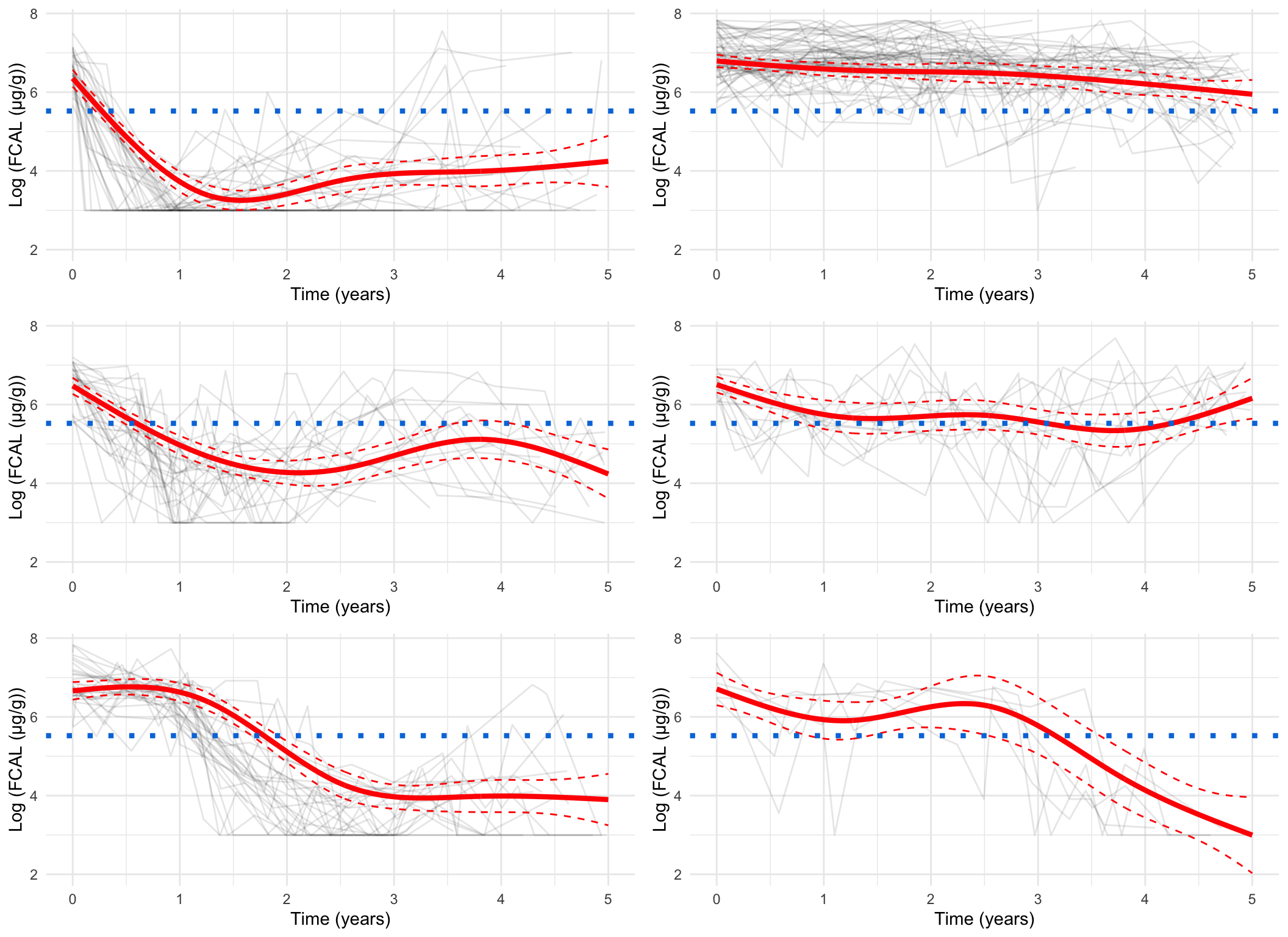
Log-scale, pprob > 0.8 only

Code

spaghetti_plot(FCcumulative,
               cubicbf.fits,
               G = 6,
               log = TRUE,
               pprob.cutoff = 0.8)

Measurement-scale, pprob > 0.8 only

Code

spaghetti_plot(FCcumulative,
               cubicbf.fits,
               G = 6,
               log = FALSE,
               pprob.cutoff = 0.8)

Model output

After considering all of the above findings, the model which assumes four clusters has been deemed the most appropriate. The summary statistics for this model can be found below. The four splines are denoted by X_{1}(t), \ldots, X_{4}(t). We use this notation in the supplementary materials for the paper.

Code

### Match notation to supp. materials
x <- cubicbf.fits[[4]]
x$Xnames <- c("Intercept", paste0("X", seq(1, 4), "(t)")) # Random effects
names(x$best) <- c(paste("Intercept class ", seq(1, 3)),# Class membership model
                   paste("Intercept class ", seq(1, 4)),# Longitudinal model
                   paste("X1(t) class ", seq (1, 4)),
                   paste("X2(t) class ", seq (1, 4)),
                   paste("X3(t) class ", seq (1, 4)),
                   paste("X4(t) class ", seq (1, 4)),
                   paste("Varcov ", seq(1, 15)),
                   "Standard error")
summary(x)

Heterogenous linear mixed model 
     fitted by maximum likelihood method 
 
hlme(fixed = value ~ ns(time, df = 4), mixture = ~ns(time, df = 4), 
    random = ~ns(time, df = 4), subject = "id", ng = ng, data = FCcumulative, 
    verbose = FALSE)
 
Statistical Model: 
     Dataset: FCcumulative 
     Number of subjects: 356 
     Number of observations: 2856 
     Number of latent classes: 4 
     Number of parameters: 39  
 
Iteration process: 
     Convergence criteria satisfied 
     Number of iterations:  20 
     Convergence criteria: parameters= 8.7e-05 
                         : likelihood= 8.1e-05 
                         : second derivatives= 1.8e-07 
 
Goodness-of-fit statistics: 
     maximum log-likelihood: -3983.49  
     AIC: 8044.97  
     BIC: 8196.1  
 
 
Maximum Likelihood Estimates: 
 
Fixed effects in the class-membership model:
(the class of reference is the last class) 

                       coef      Se    Wald p-value
Intercept class  1 -1.60714 0.60509  -2.656 0.00791
Intercept class  2 -0.97547 0.24466  -3.987 0.00007
Intercept class  3 -0.71987 0.19000  -3.789 0.00015

Fixed effects in the longitudinal model:

                       coef      Se    Wald p-value
Intercept class  1  6.63001 0.18260  36.309 0.00000
Intercept class  2  6.60767 0.10692  61.803 0.00000
Intercept class  3  6.40075 0.08792  72.805 0.00000
Intercept class  4  6.68268 0.05943 112.452 0.00000
X1(t) class  1     -0.06345 0.61580  -0.103 0.91794
X1(t) class  2     -3.02786 0.30213 -10.022 0.00000
X1(t) class  3     -2.58120 0.28225  -9.145 0.00000
X1(t) class  4     -0.32661 0.15224  -2.145 0.03192
X2(t) class  1     -1.66557 0.66716  -2.497 0.01254
X2(t) class  2     -2.43912 0.41567  -5.868 0.00000
X2(t) class  3     -0.73639 0.30260  -2.434 0.01495
X2(t) class  4     -0.76938 0.18402  -4.181 0.00003
X3(t) class  1     -4.31021 0.83955  -5.134 0.00000
X3(t) class  2     -2.38786 0.33995  -7.024 0.00000
X3(t) class  3     -4.60973 0.32173 -14.328 0.00000
X3(t) class  4     -1.29125 0.19433  -6.645 0.00000
X4(t) class  1     -1.93148 0.69759  -2.769 0.00563
X4(t) class  2     -2.65713 0.33911  -7.835 0.00000
X4(t) class  3     -0.59806 0.28348  -2.110 0.03488
X4(t) class  4     -0.21947 0.15304  -1.434 0.15155


Variance-covariance matrix of the random-effects:
          Intercept    X1(t)   X2(t)   X3(t)   X4(t)
Intercept   0.01816                                 
X1(t)       0.00354  0.69013                        
X2(t)      -0.07139 -0.20182 1.56220                
X3(t)       0.03241 -0.21967 0.67262 0.65261        
X4(t)      -0.06129 -0.19956 0.31425 0.09602 0.47886

                             coef      Se
Residual standard error:  0.77672 0.01273

Session information

R version 4.3.2 (2023-10-31)

Platform: aarch64-apple-darwin20 (64-bit)

locale: en_GB.UTF-8||en_GB.UTF-8||en_GB.UTF-8||C||en_GB.UTF-8||en_GB.UTF-8

attached base packages: grid, splines, stats, graphics, grDevices, utils, datasets, methods and base

other attached packages: DT(v.0.30), qqplotr(v.0.0.6), ggalluvial(v.0.12.5), ggdist(v.3.3.0), patchwork(v.1.1.3), htmltools(v.0.5.7), lcmm(v.2.1.0), lubridate(v.1.9.3), forcats(v.1.0.0), stringr(v.1.5.1), dplyr(v.1.1.4), purrr(v.1.0.2), readr(v.2.1.4), tidyr(v.1.3.0), tibble(v.3.2.1), ggplot2(v.3.4.4) and tidyverse(v.2.0.0)

loaded via a namespace (and not attached): tidyselect(v.1.2.0), farver(v.2.1.1), bitops(v.1.0-7), fastmap(v.1.1.1), pracma(v.2.4.4), digest(v.0.6.33), timechange(v.0.2.0), lifecycle(v.1.0.4), ellipsis(v.0.3.2), survival(v.3.5-7), magrittr(v.2.0.3), compiler(v.4.3.2), rlang(v.1.1.2), tools(v.4.3.2), utf8(v.1.2.4), yaml(v.2.3.7), knitr(v.1.45), labeling(v.0.4.3), htmlwidgets(v.1.6.3), plyr(v.1.8.9), xml2(v.1.3.5), memuse(v.4.2-3), withr(v.2.5.2), numDeriv(v.2016.8-1.1), fansi(v.1.0.5), opdisDownsampling(v.0.8.2), caTools(v.1.18.2), colorspace(v.2.1-0), scales(v.1.2.1), iterators(v.1.0.14), MASS(v.7.3-60), cli(v.3.6.1), mvtnorm(v.1.2-3), rmarkdown(v.2.25), ragg(v.1.2.6), marqLevAlg(v.2.0.8), generics(v.0.1.3), twosamples(v.2.0.1), robustbase(v.0.99-0), httr(v.1.4.7), tzdb(v.0.4.0), pander(v.0.6.5), rvest(v.1.0.3), parallel(v.4.3.2), vctrs(v.0.6.4), Matrix(v.1.6-3), jsonlite(v.1.8.7), benchmarkme(v.1.0.8), hms(v.1.1.3), systemfonts(v.1.0.5), crosstalk(v.1.2.0), foreach(v.1.5.2), jquerylib(v.0.1.4), glue(v.1.6.2), benchmarkmeData(v.1.0.4), DEoptimR(v.1.1-3), codetools(v.0.2-19), rngWELL(v.0.10-9), distributional(v.0.3.2), stringi(v.1.8.1), gtable(v.0.3.4), quadprog(v.1.5-8), randtoolbox(v.2.0.4), munsell(v.0.5.0), pillar(v.1.9.0), clisymbols(v.1.2.0), rappdirs(v.0.3.3), R6(v.2.5.1), httr2(v.1.0.0), textshaping(v.0.3.7), doParallel(v.1.0.17), evaluate(v.0.23), lattice(v.0.21-9), qqconf(v.1.3.2), Rcpp(v.1.0.11), nlme(v.3.1-163), xfun(v.0.41) and pkgconfig(v.2.0.3)

MRC Human Genetics Unit logo

Acknowledgments

This work is funded by the Medical Research Council & University of Edinburgh via a Precision Medicine PhD studentship (MR/N013166/1, to NC-C)

Author contributions

NC-C wrote the analysis. KM and CAV performed code review and contributed suggestions. KM, RM and CAV provided feedback.

Reuse

Licensed by CC BY except for the MRC Human Genetics Unit, The University of Edinburgh, and Centre for Genomic & Experimental Medicine logos or unless otherwise stated.

References

Elhakeem, Ahmed, Rachael A. Hughes, Kate Tilling, Diana L. Cousminer, Stefan A. Jackowski, Tim J. Cole, Alex S. F. Kwong, et al. 2022. “Using Linear and Natural Cubic Splines, SITAR, and Latent Trajectory Models to Characterise Nonlinear Longitudinal Growth Trajectories in Cohort Studies.” BMC Medical Research Methodology 22 (1): 68. https://doi.org/10.1186/s12874-022-01542-8.

Fornberg, Bengt, and Julia Zuev. 2007. “The Runge Phenomenon and Spatially Variable Shape Parameters in RBF Interpolation.” Computers & Mathematics with Applications 54 (3): 379–98. https://doi.org/https://doi.org/10.1016/j.camwa.2007.01.028.

Proust-Lima, Cécile, Viviane Philipps, and Benoit Liquet. 2017. “Estimation of Extended Mixed Models Using Latent Classes and Latent Processes: The R Package lcmm.” Journal of Statistical Software 78 (2): 1–56. https://doi.org/10.18637/jss.v078.i02.

Citation

BibTeX citation:

@article{constantine-cooke2023,
  author = {Nathan Constantine-Cooke and Karla Monterrubio-Gómez and
    Nikolas Plevris and Lauranne A.A.P. Derikx and Beatriz Gros and
    Gareth-Rhys Jones and Riccardo E. Marioni and Charlie W. Lees and
    Catalina A. Vallejos},
  publisher = {Elsevier},
  title = {Longitudinal {Fecal} {Calprotectin} {Profiles} {Characterize}
    {Disease} {Course} {Heterogeneity} in {Crohn’s} {Disease}},
  journal = {Clinical Gastroenterology and Hepatology},
  date = {2023-11-24},
  url = {https://www.cghjournal.org/article/S1542-3565(23)00234-3/},
  doi = {10.1016/j.cgh.2023.03.026},
  issn = {1542-3565},
  langid = {en}
}

For attribution, please cite this work as:

Nathan Constantine-Cooke, Karla Monterrubio-Gómez, Nikolas Plevris, Lauranne A.A.P. Derikx, Beatriz Gros, Gareth-Rhys Jones, Riccardo E. Marioni, Charlie W. Lees, and Catalina A. Vallejos. 2023. “Longitudinal Fecal Calprotectin Profiles Characterize Disease Course Heterogeneity in Crohn’s Disease.” Clinical Gastroenterology and Hepatology, November. https://doi.org/10.1016/j.cgh.2023.03.026.