Preprocessing
Introduction
This page details preprocessing steps undertaken prior to model fitting. These steps include examining data quality, performing data cleaning, and deriving the study cohort.
The biomarker (FC and CRP) data used in this pipeline have been primarily obtained from TRAK, a system used by NHS Lothian for the electronic ordering of laboratory tests. However, we also use phenotyping data manually curated by the Lees group for previous studies (see Jenkinson et al. (2020)).
Prior to this report, all subject CHI (community health index) numbers, which uniquely identifies a patient when they interact with NHS Scotland services, were pseudoanonymised. Each CHI has been replaced with a unique random number.
Inclusion/exclusion criteria definitions
The inclusion criteria for this study can broadly be categorised into two classifications: baseline and longitudinal. Baseline criteria can be applied using information known at diagnosis whilst longitudinal criteria are based on biomarker measurements taken over time.
The longitudinal criteria for each biomarker (FC and CRP) are considered independently. If a subject meets the below criteria for FC but not CRP, then only the FC for the subject will be modelled and vice versa.
Diagnosis of Inflammatory bowel disease
As inflammatory bowel disease (IBD) is the disease of interest for this study, subjects are required to have a confirmed diagnosis of either Crohn’s disease, ulcerative colitis, or inflammatory bowel disease unclassified.
Diagnosis date
Study subjects are required to have been diagnosed with IBD between January 2008 and December 2017. The lower bound is required as FC tests were not typically used for disease monitoring prior to this period and were instead used only for diagnostic purposes. The upper bound is required to ensure subjects have the opportunity to have at least five years of follow-up. The most recent FC observation in this dataset is January 2023 which informed when deciding upon this cut-off.
Diagnostic measurement
We require study subjects to have a biomarker measurement taken ±90 days of reported date of diagnosis.
At least three non-censored measurements
To ensure stability and interpretability, study subjects are also required to have at three non-censored biomarker measurements taken across follow-up. Like most biomarkers, the biomarkers used in this study are subject to censoring. However, these censored observations make it impossible to detect changes over time and we therefore do not wish to be reliant on censored observations.
Datasets
Code
if (file.exists("/.dockerenv")) { # Check if running in Docker
  # Assume igmm/Vallejo-predict/libdr/ is passed to the data volume
  prefix <- "data/"
} else {
  # Assume running outside of a Docker container and the IGC(/IGMM) datastore is
  # mounted at /Volumes
  prefix <- "/Volumes/igmm/cvallejo-predicct/libdr/"
}

fcal.pheno <- read.csv(file.path(prefix, "2024-10-03/fcal-cleaned.csv"))

# Extract from TRAK which also now introduces CRP.
labs <- read.csv(file.path(prefix, "2024-10-03/markers-cleaned.csv"))
fcal <- subset(labs, TEST == "f-Calprotectin-ALP")

# Add sex and diagnosis type from fcal.pheno
fcal <- fcal.pheno %>%
  distinct(ids, .keep_all = TRUE) %>%
  select(ids, sex, diagnosis, diagnosis_date) %>%
  merge(x = fcal, by = "ids", all.x = TRUE, all.y = FALSE)

crp <- subset(labs, TEST == "C-Reactive Prot")
updated <- read.csv(file.path(prefix, "2024-10-03/allPatientsNathanCleaned.csv"))
outcomes <- read.csv(file.path(prefix, "2024-10-03/cd-cleaned.csv"))

non.ibd <- read.csv(file.path (prefix, "2024-10-24/non-ibd.csv"))
Multiple datasets are used in this report with varying degrees of previous curation.
-
markers.csvis a 2024 extraction from TRAKcare describing 286294 test results (FC: 60866; CRP: 225428). Each row represents a test result with columns indicating the corresponding subject ID, the test type (FC or CRP), the time of the test, and the test result. This dataset contains the most recent data out of the other datasets. However, there has been no manual curation of these data, and no information about the patient’s characteristics are available (other than their ID). -
fcal-cleaned.csvdoes not describe CRP data. However, these data have been curated by the Lees group. In addition to 60866 FC test results, each row also provides the sex, IBD type, date of diagnosis, and date of death (if applicable) for the corresponding subject. -
allPatientsNathanCleaned.csvprovides sex, IBD type, and diagnosis date for most (but not all) subjects inlabs.csvnot described byfcal-cleaned.csv. -
cd-cleaned.csvdescribes CD patient data (n = 1753). In addition to the same basic patient characteristic variables in other datasets, this dataset also describes surgical outcomes and biologic treatments prescribed to the subject. -
non-ibd.csvdescribes subjects who were found to not have IBD during the phenotyping process. This dataset is used to remove subjects who do not have IBD from the analysis.
The “cleaned” in the above file names refers to the CHI numbers having been replaced. No further processing of the data has been undertaken for this study prior to the steps outlined in this report.
Subject data
We will create a “dictionary” which, for each subject, lists their subject ID, their IBD type, and their date of diagnosis. In addition to ensuring inclusion criteria are met, date of diagnosis will be used to retime all biomarker measurements of a subject such that t=0 corresponds to their diagnosis date. IBD types are used to test if clusters are enriched by IBD type and may be used to adjust the clustering.
There are multiple potential sources for date of diagnosis and IBD type: the CD outcomes dataset, a demographics dataset maintained by the Lees group, and a raw TRAK extraction. For every subject listed in at least one of these datasets, we have tried to extract their date of diagnosis and diagnosis type. We have assumed a hierarchy of datasets where manually curated datasets are preferred for extracting data over a dataset generated with minimal human involvement.
Diagnosis and diagnosis date
Code
ids <- unique(c(outcomes$ids, fcal$ids, updated$ids))
diagnosis <- character()
date.of.diag <- character()
for (id in ids) {
  if (id %in% outcomes$ids) {
    # Outcomes data only contains CD subjects
    diagnosis <- c(diagnosis, "Crohn's Disease")
    date.of.diag <- c(
      date.of.diag,
      subset(outcomes, ids == id)$diagnosisDate
    )
  } else if (id %in% updated$ids) {
    diagnosis <- c(diagnosis, subset(updated, ids == id)[1, "diagnosis"])
    date.of.diag <- c(
      date.of.diag,
      subset(updated, ids == id)[1, "diagnosisDate"]
    )
  } else if (id %in% fcal$ids) {
    diagnosis <- c(diagnosis, subset(fcal, ids == id)[1, "diagnosis"])
    date.of.diag <- c(
      date.of.diag,
      subset(fcal, ids == id)[1, "diagnosis_date"]
    )
  } else {
    diagnosis <- c(diagnosis, "Unknown")
    date.of.diag <- c(
      date.of.diag,
      "Unknown"
    )
  }
}

dict <- data.frame(
  ids = ids,
  diagnosis = diagnosis,
  date.of.diag = fix_date_char(date.of.diag)
)


rm(id, ids, diagnosis, date.of.diag) # clean up
dict <- fix_date_df(dict, "date.of.diag")
Before filtering by inclusion/exclusion criteria, there are 7 individuals for which a diagnostic date is missing. However, 0 missing values are observed for diagnosis (IBD type).
As can be seen in the below table, two spellings of Crohn’s disease (with and without an apostrophe (’)) and three names for IBDU are used. There are also subjects reported to not have IBD. These will be removed, leaving 10153 subjects included in the subsequent analyses.
Code
| Diagnosis |
|---|
| Crohn’s Disease |
| Inflamatory Bowel Disease - Unknown Subtype |
| Crohns Disease |
| Ulcerative Colitis |
| Inflamatory Bowel Disease |
| IBDU |
| Not IBD |
The Crohn’s disease and IBDU names have been standardised (IBDU, Inflammatory Bowel Disease, Inflammatory Bowel Disease - Unknown Subtype are assumed to be equivalent). The subject reported to not have IBD has been removed.
Code
dict$old <- dict$diagnosis
dict$diagnosis <- plyr::mapvalues(
  dict$diagnosis,
  from = c(
    "Crohns Disease",
    "Inflamatory Bowel Disease",
    "Inflamatory Bowel Disease - Unknown Subtype"
  ),
  to = c(
    "Crohn's Disease",
    "IBDU",
    "IBDU"
  )
)

kable(addmargins(table(dict$diagnosis, dict$old), margin = 2))
dict$old <- NULL| Crohn’s Disease | Crohns Disease | IBDU | Inflamatory Bowel Disease | Inflamatory Bowel Disease - Unknown Subtype | Ulcerative Colitis | Sum | |
|---|---|---|---|---|---|---|---|
| Crohn’s Disease | 2471 | 1328 | 0 | 0 | 0 | 0 | 3799 |
| IBDU | 0 | 0 | 1 | 242 | 841 | 0 | 1084 |
| Ulcerative Colitis | 0 | 0 | 0 | 0 | 0 | 5270 | 5270 |
Age and sex
Code
# Merge with fcal to add sex information
dict <- fcal.pheno[, c("ids", "sex")] %>%
  distinct(ids,
    .keep_all = TRUE
  ) %>%
  merge(x = dict, by = "ids", all.x = TRUE, all.y = FALSE)

# Update NA sex if sex available from updated
dict <- merge(dict,
  updated[, c("ids", "sex")],
  by = "ids",
  all.x = TRUE,
  all.y = FALSE
)

for (i in seq_len(nrow(dict))) {
  if (is.na(dict[i, "sex.x"]) && !is.na(dict[i, "sex.y"])) {
    dict[i, "sex.x"] <- dict[i, "sex.y"]
  }
}

dict$sex <- dict$sex.x
dict$sex.x <- dict$sex.y <- NULL

# Add age at IBD diagnosis
updated <- fix_date_df(updated, "diagnosisDate")
updated$age <- with(updated, year(diagnosisDate) - dateOfBirth)
dict <- merge(dict,
  updated[, c("ids", "age")],
  by = "ids",
  all.x = TRUE,
  all.y = FALSE
)
Note that there 7 individuals for which age at diagnosis is missing (this is due to missing diagnostic dates). However, there are 0 individuals for which sex is missing.
Date of death
Code
dict <- merge(dict,
  updated[, c("ids", "death")],
  by = "ids",
  all.x = TRUE,
  all.y = FALSE
) %>%
  rename(date.of.death = death)

dict <- fix_date_df(dict, "date.of.death")
Date of death information is available for 1136 individuals. We assume that all remaining individuals have not died by the date of data extraction.
Exclusion criteria according to diagnosis and date of diagnosis
Date of diagnosis in an integral aspect of the inclusion criteria and also used to retime biomarker measurements.
Firstly, we remove 7 individuals with a missing date of diagnosis.
Code
dict <- dict[!is.na(dict$date.of.diag), ]This leaves 10146 for subsequent analyses.
Code
# no. subjects over upper bound
max_fup <- max(labs$COLLECTION_DATE)
max_fup <- as.Date(max_fup)
n.upper <- nrow(subset(dict, max_fup - date.of.diag < 5 * 365.25))

# no. subjects under lower bound
n.lower <- nrow(subset(dict, year(date.of.diag) < 2008))

# subset to subjects meeting the criteria.
dict <- subset(dict, max_fup - date.of.diag >= 5 * 365.25)
dict <- subset(dict, year(date.of.diag) >= 2008)
As described in the inclusion/exclusion criteria section, the inclusion criteria considers upper and lower bounds for the diagnostic dates. In this case, we only consider subjects diagnosed from 1 January 2008 and before 13 August 2019 (this ensures individuals can be followed up by at least 5 year by the time of the last longitudinal measument obtained for the cohort; 2024-08-13). As such, subjects who do not meet this criteria will be excluded. 77 subjects were diagnosed on 13 August 2019 or later and were removed, and 5588 subjects were diagnosed prior to 2008 and were likewise removed. This results in a cohort size of 4481 subjects.
Exploration
We now explore date of diagnosis to ensure data quality is at a suitable standard.
Year of diagnosis
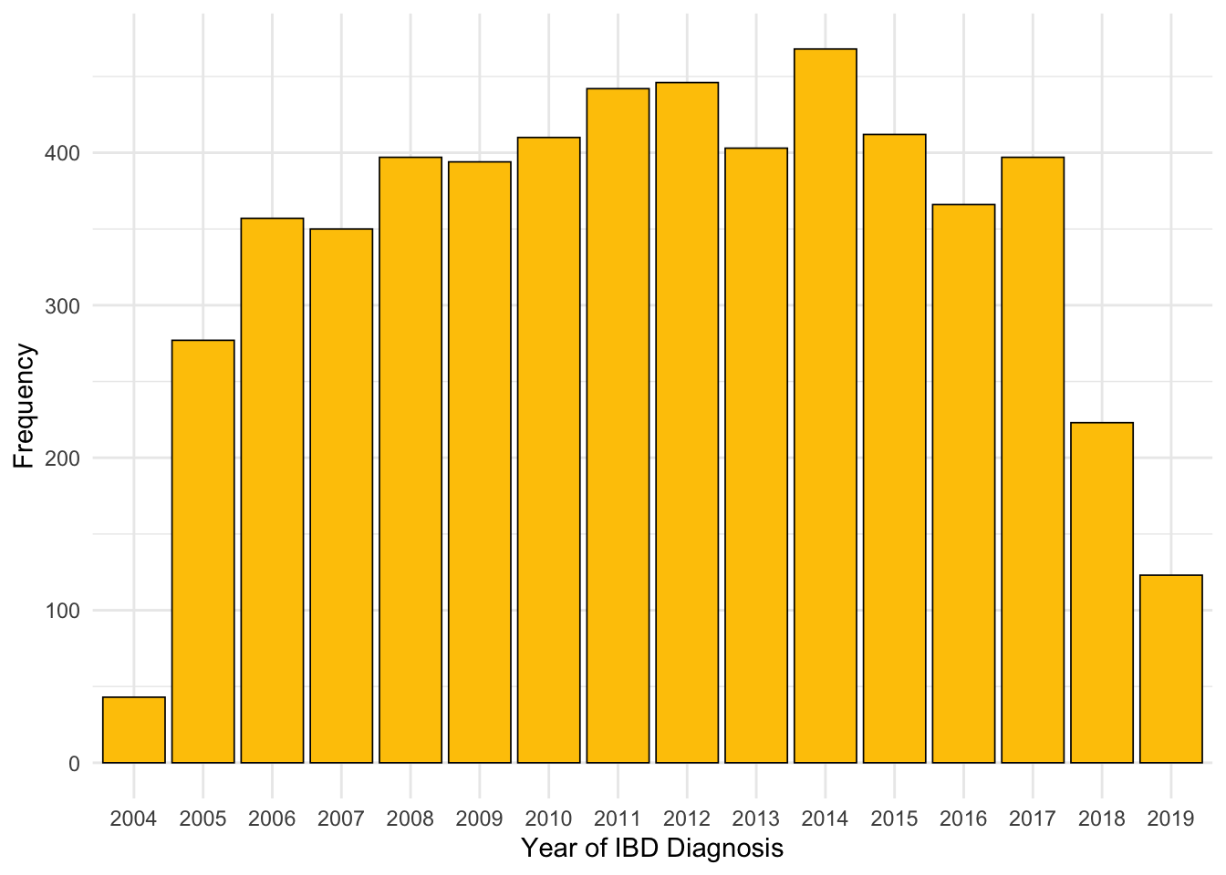
From Figure 1, we can see the number of IBD diagnoses each year is relatively static with the exception of 2004 and 2005. The former describes only three months of the year, and incidence was likely still increasing across both of these two years. Jones et al. (2019) found IBD incidence from 2008 onwards to be consistent over time for patients diagnosed by NHS Lothian which is in agreement with our findings.
Code
dict %>%
  ggplot(aes(x = year(date.of.diag))) +
  geom_histogram(fill = "#B8F2E6", color = "black", binwidth = 1) +
  theme_minimal() +
  xlab("Year of IBD diagnosis") +
  ylab("Frequency")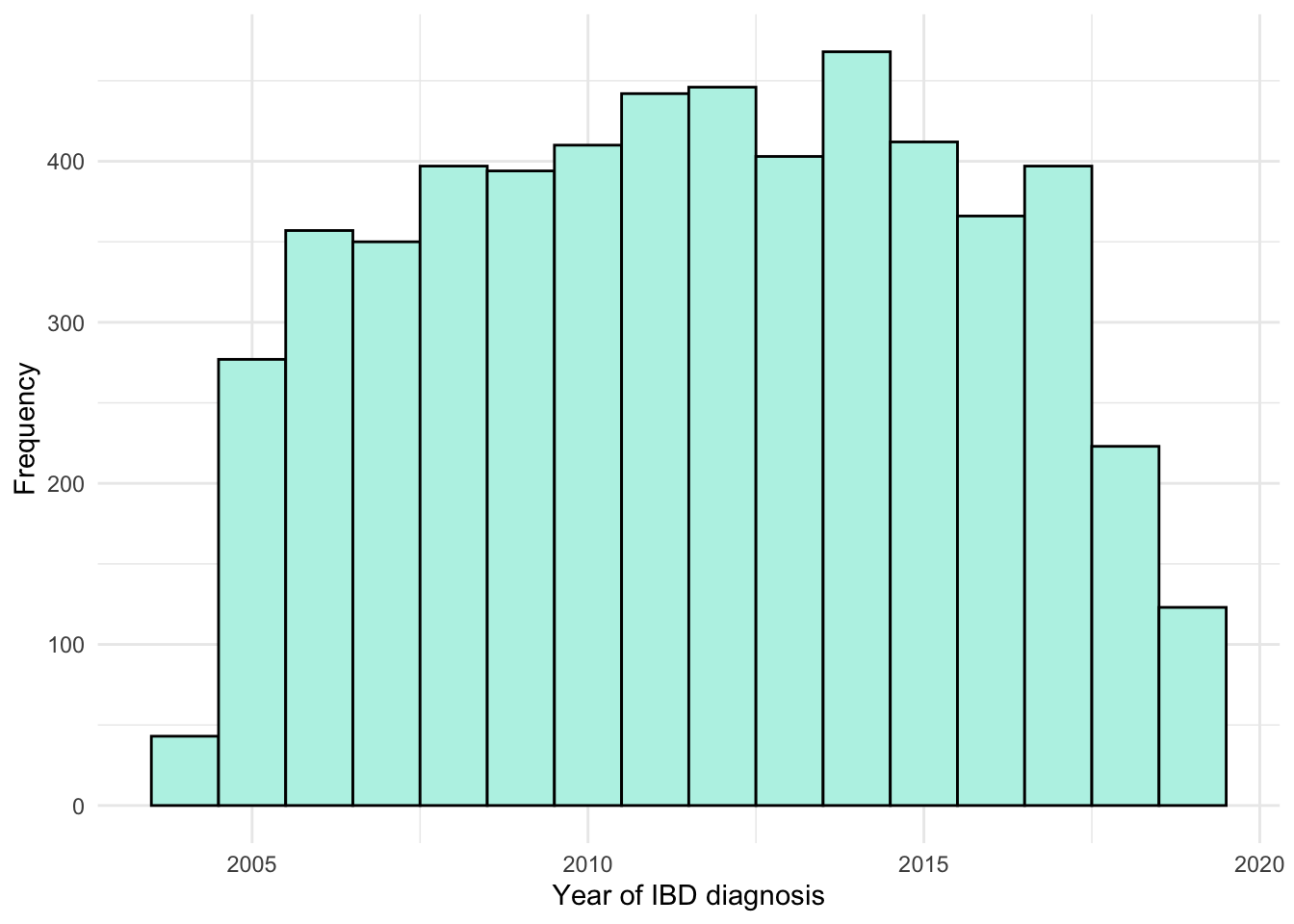
Month of diagnosis
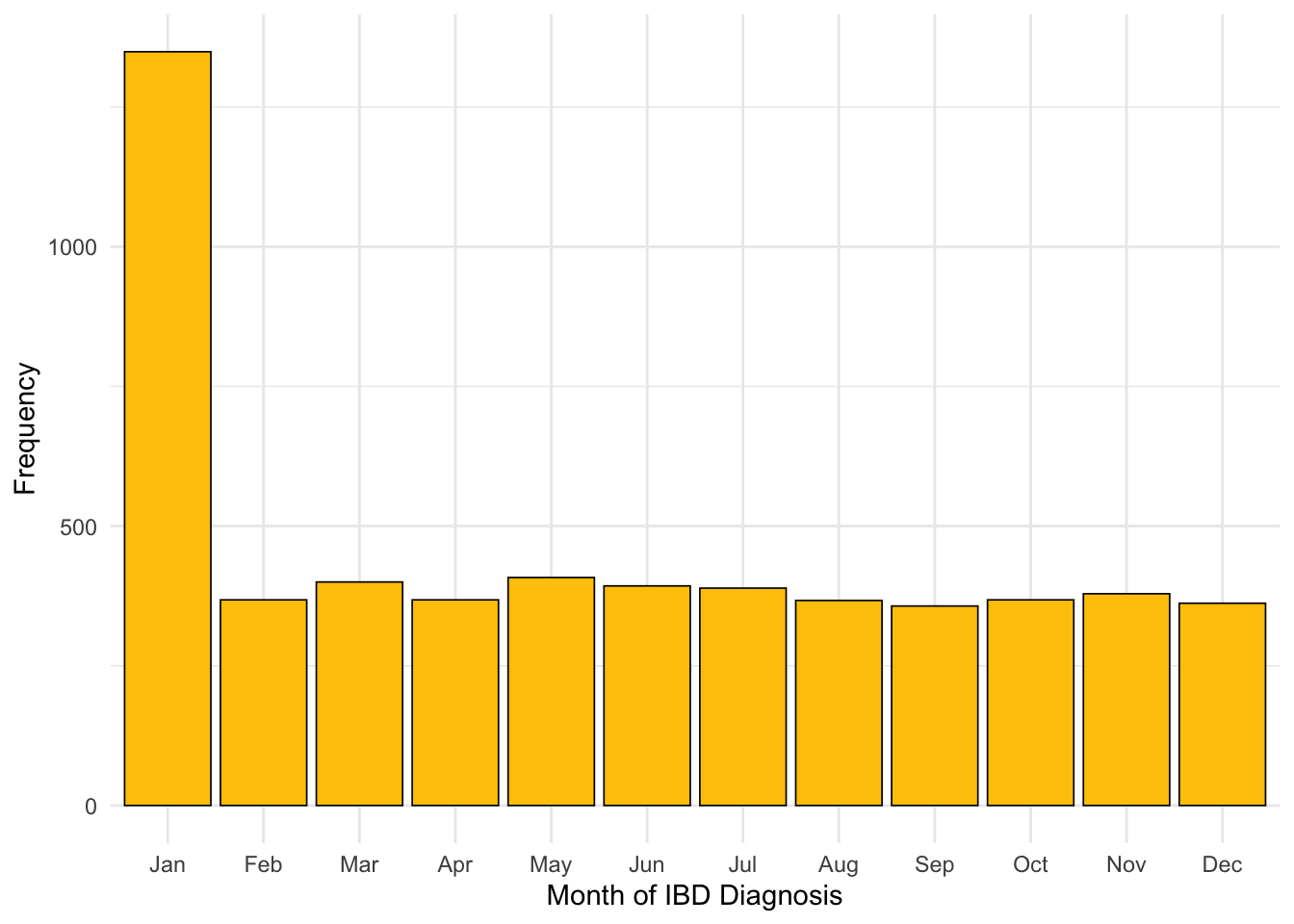
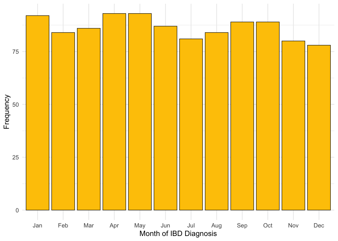
It appears there are subjects for whom only year of diagnosis was available. This has resulted in the 1st of January for that year being recorded as the date of diagnosis for that subject. As such, far more diagnoses are reported in January than in other months (Figure 3). There are 707 subjects reported to have been diagnosed on New Year’s day .
If a subject’s exact date of diagnosis is not known, then this is most likely because the subject was not diagnosed by NHS Lothian. Instead, the date of diagnosis would have needed to be recalled by the subject which introduces the inaccuracy observed.
As subjects are require a diagnostic biomarker measurement to be available within 90 days of reported date of diagnosis to be included in this study and patients diagnosed outside of NHS Lothian will not have a biomarker test result available within this period, the effect on our study should be minimal. However, we will revisit month of diagnosis after filtering by existence of diagnostic biomarker measurements to confirm our assumption.
Code
Code
Code
diag.ts <- dict %>%
  mutate(
    date.of.diag.month =
      as.Date(paste0(format(date.of.diag, "%Y-%m"), "-01"), format = "%Y-%m-%d")
  ) %>%
  group_by(date.of.diag.month) %>%
  summarise(count = n()) %>%
  ungroup()

diag.ts %>%
  ggplot(aes(x = as.Date(date.of.diag.month, "%Y-%m"), y = count, group = 1)) +
  geom_line() +
  xlab("Diagnosis date") +
  ylab("Number of diagnosis") +
  scale_x_date(date_labels = "%Y-%m") +
  theme_minimal()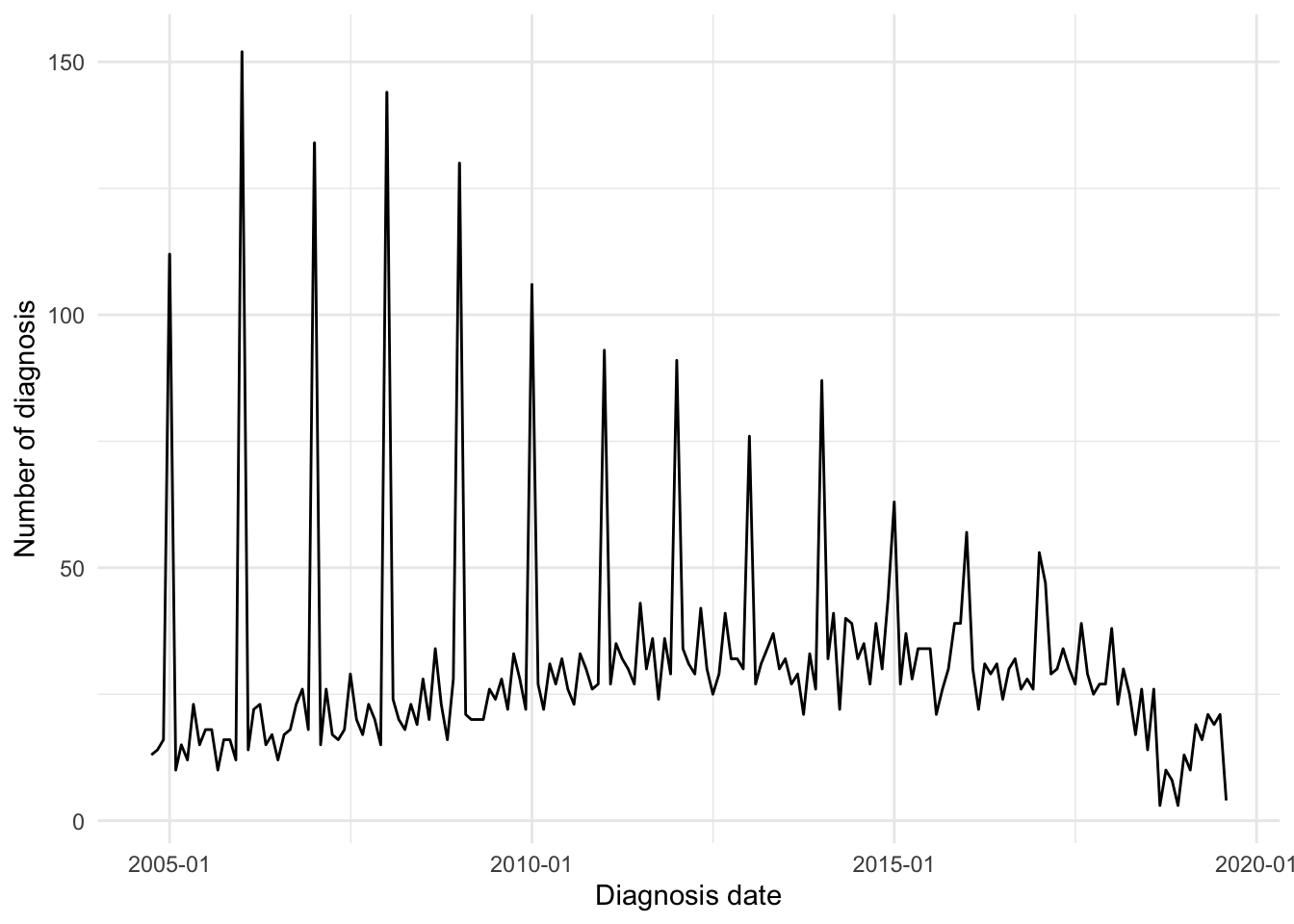
Faecal calprotectin
Faecal calprotectin (FC), a marker of intestinal inflammation, has been obtained from two datasets. The first dataset has been curated by members of the Lees group whilst the second dataset is a direct extract from TRAK, a patient monitoring system used by NHS Lothian.
Incorporating later extract
Data from these datasets has been merged and duplicates of data (same subject ID, measurement date, and recorded value) were removed. We also reduced the FC dataset to only describe subjects for whom IBD type and date of diagnosis are available for.
For the TRAK extract, times for test results are given in datetime format (where both date and time of the day are provided). The times have been dropped as this degree of granularity is not required. Duplicate tests (same id, date and test value) are removed here.
Code
fcal <- fcal[, c(
  "ids",
  "COLLECTION_DATE",
  "TEST_DATA",
  "sex",
  "diagnosis",
  "diagnosis_date"
)]

# Subset to only include those that passed the earlier inclusion/exclusion
fcal <- subset(fcal, ids %in% dict$ids)

# Collection dates include collection times which are not required. Discarding.

fcal$COLLECTION_DATE <- readr::parse_date(
  stringr::str_split_fixed(fcal$COLLECTION_DATE, " ", n = 2)[, 1],
  format = "%Y-%m-%d"
)

colnames(fcal)[1:3] <- c("ids", "calpro_date", "calpro_result")

fcal <- subset(fcal, ids %in% dict$ids)
fcal <- fcal %>%
  select(-diagnosis)

fcal <- merge(fcal,
  dict[, c("ids", "diagnosis", "date.of.diag")],
  by = "ids",
  all.x = TRUE
)
Pre-processing of test results
Code
## Some values cannot be directly coerced as numeric

fcal$calpro_result <- plyr::mapvalues(
  fcal$calpro_result,
  from = c(
    "<20",
    "<25",
    "<50",
    ">1250",
    ">2500",
    ">3000",
    ">6000"
  ),
  to = c(
    "20",
    "25",
    "50",
    "1250",
    "2500",
    "3000",
    "6000"
  )
)

# Here, values that cannot be converted into a numeric value will be excluded
# (they are converted to NA)
fcal$calpro_result <- as.numeric(fcal$calpro_result) # Remove error codes
fcal <- fcal[!is.na(fcal[, "calpro_result"]), ]

# Apply limits of detection
fcal[fcal[, "calpro_result"] < 20, "calpro_result"] <- 20
fcal[fcal[, "calpro_result"] > 1250, "calpro_result"] <- 1250
FC data can be both left and right censored. FC recorded as “<20” were mapped to “20”. FC recorded as “>1250”, “>2500”, or “>6000” were all mapped to “1250”. Any FC tests given an error code (e.g. marked as an insufficient sample by the laboratory) have been removed.
The lower limit of detection is <20 \mu g/g (20 \mu g of calprotectin per g of stool). By reducing the upper limit, it is possible to run more tests in parallel. As a higher throughput has been required over time, the upper threshold for tests has become lower. Initially test results over 6000 \mu g/g were censored, then 2500 \mu g/g and now 1250 \mu g /g is the upper limit for FC tests. This change has resulted in minimal impact in clinics as 1250 \mu g/g is still considered a high result. However, this change has potential implications for research.
Code
fcal %>%
  ggplot(aes(x = calpro_result)) +
  geom_density(
    linewidth = 0.8,
    alpha = 0.5,
    fill = "#9FD8CB",
    color = "#517664"
  ) +
  theme_minimal() +
  theme(axis.text.y = element_blank()) +
  xlab("FCAL (µg/g)") +
  ylab("Density") +
  geom_vline(xintercept = 250, colour = "red")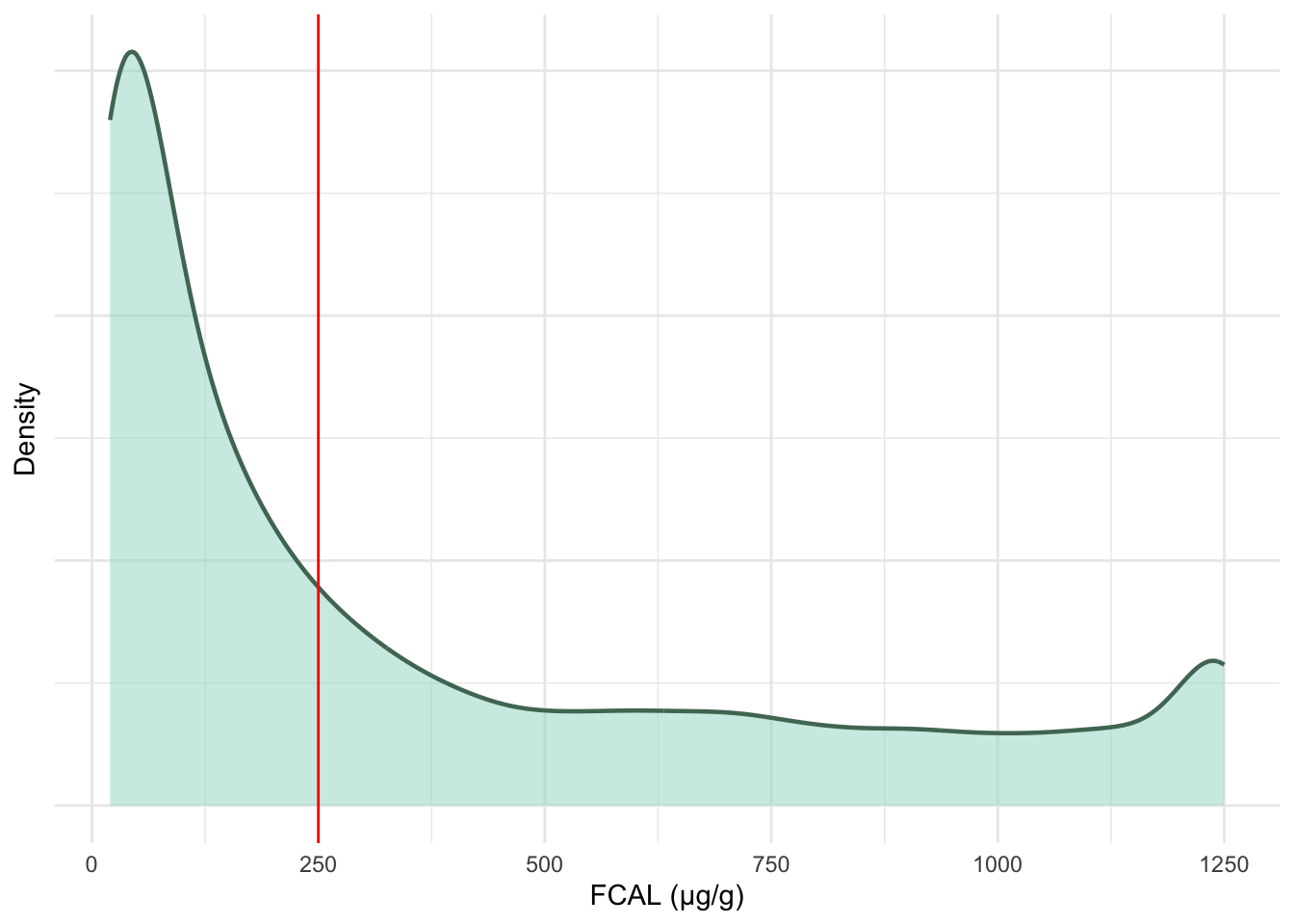
FC test results on the original measurement scale are heavily right-skewed towards 100 \mu g/g. These data will be log transformed- resulting in the multi-modal distribution seen in Figure 5.
Code
fcal %>%
  ggplot(aes(x = log(calpro_result))) +
  geom_density(
    linewidth = 0.8,
    alpha = 0.5,
    fill = "#9FD8CB",
    color = "#517664"
  ) +
  theme_minimal() +
  theme(axis.text.y = element_blank()) +
  xlab("log(FCAL (µg/g))") +
  ylab("Density") +
  geom_vline(xintercept = log(250), colour = "red")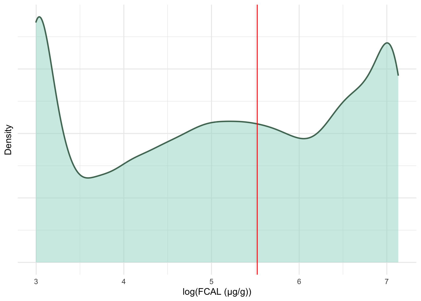
Removal of duplicate FCAL measurements
Code
duplicated.ids <- c()

for (id in unique(fcal$ids)) {
  sub.fcal <- subset(fcal, ids == id) # Get FC data for a subject
  sub.fcal <- sub.fcal[order(sub.fcal$calpro_date), ] # Order by dates
  time.diff <- diff(sub.fcal$calpro_date) # Find time between ordered dates
  value.diff <- diff(sub.fcal$calpro_result) # Find difference in observed values
  # If two measurements are within 10 days of each other and have the same value
  if (any(time.diff <= 10 & value.diff == 0)) {
    duplicated.ids <- c(duplicated.ids, id)
    # Remove suspected duplicates (taking into account difference is lagged)
    sub.fcal <- sub.fcal[c(TRUE, !(time.diff <= 10 & value.diff == 0)), ]
    # Remove data for subject with duplicates
    fcal <- subset(fcal, ids != id)
    # Add non duplicated data back
    fcal <- rbind(fcal, sub.fcal)
  }
}
Given FC was retrospectively collected from observational data, it is possible duplicate tests have been recorded in the extract. As it is NHS Lothian policy to not test FC days apart, we can assume that any tests with the same observation within a small time frame are likely to be duplicates. This may occur when collection dates and testing dates have been used interchangeably.
If a subsequent FC test for a subject was dated within 10 days of a previous test and has the same observed value, this observation was dropped.
Retiming - part 1
Time of FC measurements were retimed and scaled to be the number of years since IBD diagnosis.
Code
# Dates have already been converted to Date class by fix_date_char() for dict
fcal$calpro_time <- as.numeric(fcal$calpro_date - fcal$date.of.diag) / 365.25

fcal %>%
  ggplot(aes(x = calpro_time, y = log(calpro_result), color = factor(ids))) +
  geom_line(alpha = 0.2) +
  geom_point(alpha = 0.6) +
  theme_minimal() +
  scale_color_manual(values = viridis::viridis(length(unique(fcal$ids)))) +
  guides(color = "none") +
  xlab("Time (years)") +
  ylab("Log(FCAL (µg/g))") +
  ggtitle("")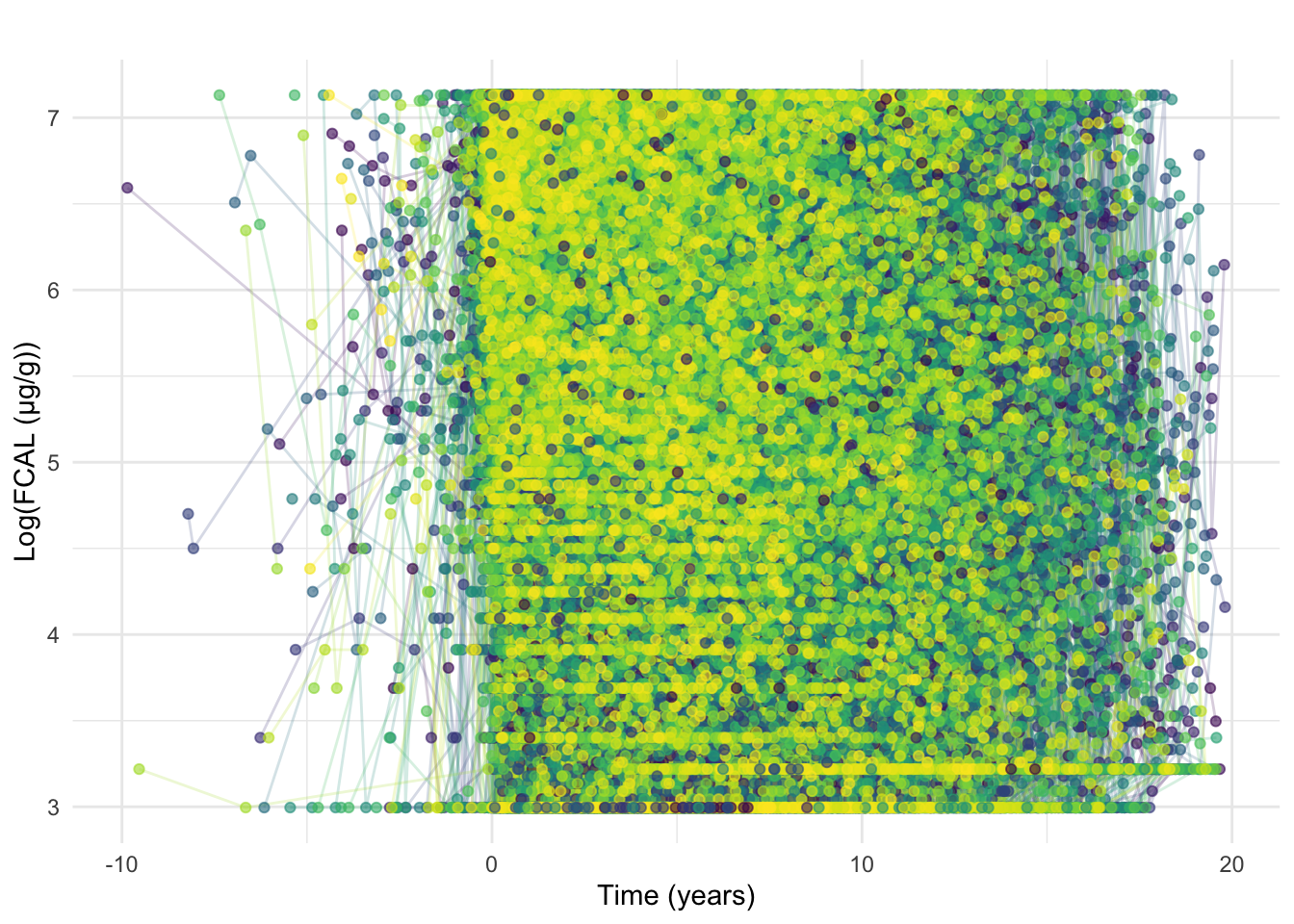
After retiming, it is clear some FC observations are earlier than diagnosis and in some cases substantially earlier (Figure 6). Tests taken close to the reported date of diagnosis are likely “early” as a result of diagnostic delay whereas tests from much earlier were likely requested due to other conditions.
As such, FC results earlier than 90 days prior to diagnosis will be discarded. If a subject has an FC within 90 days before diagnosis, then all of their FC tests will be retimed such that their earliest FC within this period is equal to 0 and all later measurements are shifted accordingly to maintain the same differences between measurement times.
Code
fcal <- subset(fcal, calpro_time >= -0.25)Inclusion/exclusion: removal of subjects without a diagnostic FC test
As indicated in our inclusion/exclusion criteria, we reduce the dataset to only subjects with a diagnostic FC. This equates to subjects with at least one FCAL measurement within 3 months of diagnosis t \leq 0.25.
After this exclusion, 1554 subjects remain in the data.
659 subjects which were excluded due to not having a diagnostic FC had a reported date of diagnosis of 1st January. Only year of diagnosis was likely available for these subjects.
Code
##The following code is used to save the cleaned data generated so far.

diag.time <- c()
fc.ids <-  unique(fcal$ids)

for (id in fc.ids) {
  temp <- subset(fcal, ids == id)
  temp <- temp[order(temp$calpro_time), ]
  diag.time <- c(diag.time, temp[1, "calpro_time"])
}


fc.dist <- data.frame(ids = fc.ids, diagnostic = diag.time)

if (!dir.exists(paste0(prefix, "processed"))) {
  dir.create(paste0(prefix, "processed"))
}

saveRDS(fc.dist, paste0(prefix, "processed/fc-diag-dist.RDS"))
Retiming - part 2
Here, we show the distribution of the diagnostic FCAL measurements with respect to diagnosis date (in days).
Code
p <- fcal %>%
  group_by(ids) %>%
  filter(calpro_time == min(calpro_time)) %>%
  ggplot(aes(x = calpro_time * 365.25)) +
  geom_density(fill = "#20A39E", color = "#187370") +
  theme_minimal() +
  labs(
    y = "Density",
    x = "Time from diagnosis to first faecal calprotectin (days)"
  ) +
  geom_vline(xintercept = 0, linetype = "dashed", color = "red")

ggsave("plots/fc-diagnostic-dist.png",
  p,
  width = 16 * 2 / 3,
  height = 6,
  units = "in"
)
Although most diagnostic measurements were observed around the recorded diagnosis time (near zero), this is not always the case. As such, we decided to retime measurements/diagnosis time as described above (i.e. time = 0 matches the time of first available FCAL measurement). This is only applied to individuals for which the first available CRP is prior to the recorded diagnosis time.
Code
[1] 1554Code
fcal %>%
  ggplot(aes(x = calpro_time, y = log(calpro_result), color = factor(ids))) +
  geom_line(alpha = 0.2) +
  geom_point(alpha = 0.6) +
  theme_minimal() +
  scale_color_manual(values = viridis::viridis(length(unique(fcal$ids)))) +
  guides(color = "none") +
  xlab("Time (years)") +
  ylab("Log(FCAL (µg/g))") +
  ggtitle("")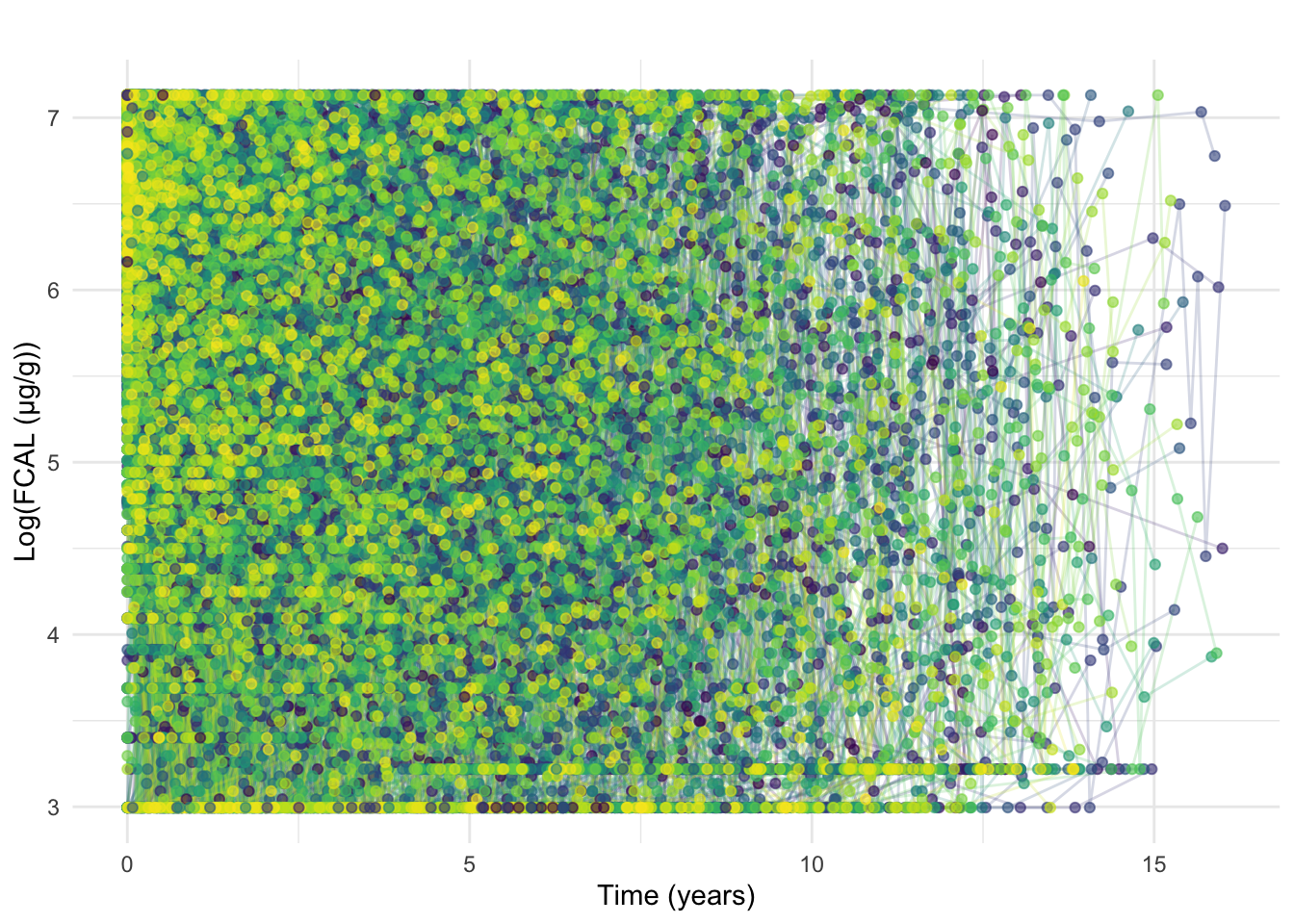
At this stage, we also exclude FCAL measurements recorded beyond 7 years post diagnosis.
At this point, the data contains 11582 FCAL measurements across all 1554 individuals.
Inclusion/exclusion: a minimum number of FCAL measurements
Here, we summarise the number of observations per individual (with and without considering censored values) as well as length of follow-up. The latter is defined as the difference (in years) between diagnosis time and the time of the latest FCAL measurement.
Code
countsDF <- fcal %>%
  group_by(ids) %>%
  summarise(
    n.total = n(),
    censored.left = sum(calpro_result == 20),
    censored.right = sum(calpro_result == 1250),
    n.noncensored = n.total - censored.left - censored.right,
    n.negtime.nondiag = sum(calpro_time != 0 & calpro_date - date.of.diag < 0),
    followup = max(calpro_time)
  )
Code
p1 <- countsDF %>%
  ggplot(aes(x = n.total)) +
  geom_histogram(color = "black", fill = "#5BBA6F", binwidth = 1) +
  theme_minimal() +
  ylab("Count") +
  xlab("Measurements per subject")
p2 <- countsDF %>%
  ggplot(aes(x = followup)) +
  geom_histogram(color = "black", fill = "#5BBA6F", binwidth = 1) +
  theme_minimal() +
  ylab("Count") +
  xlab("Follow-up (years)")
p3 <- countsDF %>%
  ggplot(aes(y = n.total, x = followup)) +
  geom_hex() +
  xlab("Follow-up (years since diagnosis)") +
  ylab("Number of FC measurements") +
  theme_minimal() +
  labs(fill = "Count")

p1 + p2 + p3 + plot_annotation(tag_levels = "A")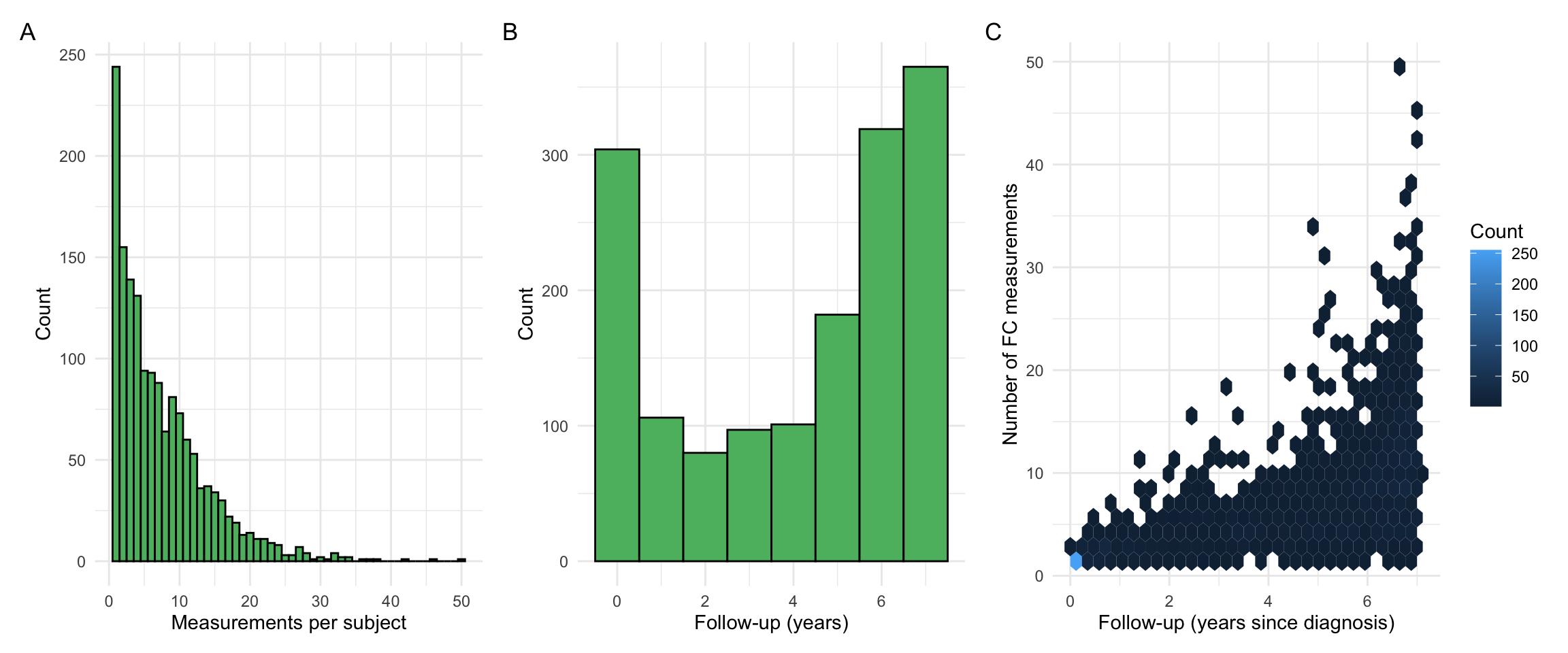
Summary observations:
- The number of FC measurements per subject is skewed towards low values. However, there are also subjects with many FC observations. These subjects were investigated and found to often have a complex disease course, such as acute severe ulcerative colitis, and required close monitoring as a result.
- We do not directly require a minimum follow-up for a subject as this may bias our findings. For example, UC patients who undergo a proctocolectomy (surgical removal of the colon and rectum) are less likely to have FC measurements after their surgery than patients who did not require surgery. By applying criteria based on follow-up, we could indirectly exclude subjects based on disease outcomes.
- However, the requirement of at least 3 FCAL measurements (within 7 years from diagnosis) will indirectly remove individuals with a very short follow-up time.
Note that our inclusion criteria requires at least 3 non-censored FCAL measurements per individual. As such, censoring needs to be taken into account before applying filtering out individuals.
Code
p1 <- countsDF %>%
  ggplot(aes(x = n.noncensored)) +
  geom_histogram(color = "black", fill = "#5BBA6F", binwidth = 1) +
  theme_minimal() +
  ylab("Count") +
  xlab("Number of non-censored measurements per subject")

p2 <- countsDF %>%
  ggplot(aes(y = n.noncensored, x = followup)) +
  geom_point(color = "#FF4F79", size = 2) +
  xlab("Follow-up (years since diagnosis)") +
  ylab("Number of non-censored FCAL measurements") +
  theme_minimal() +
  geom_hline(yintercept = 3)

p1 + p2 + plot_annotation(tag_levels = "A")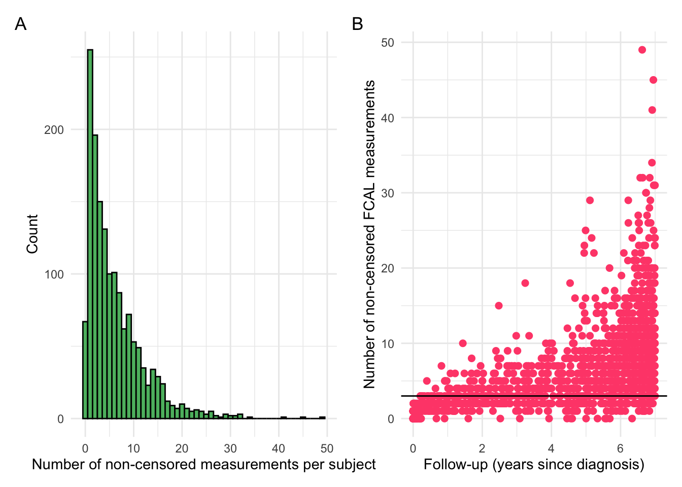
Code
# Number of individuals with at least 3 FCAL measurements
sum(countsDF$n.total >= 3)
[1] 1155Code
# Number of individuals with at least 3 non-censored FCAL measurements
sum(countsDF$n.noncensored >= 3)
[1] 1036Code
# Number of individuals with at least 3 non-censored FCAL measurements after
# discarding non-diagnostic values with negative calpro_time
sum(countsDF$n.noncensored - countsDF$n.negtime.nondiag >= 3)
[1] 1028The following is used to select individuals with at least 3 non-censored FCAL measurements.
Code
[1] 1036This leaves a cohort with 1036 individuals.
Code
p1 <- countsDF %>%
  subset(n.noncensored >= 3) %>%
  ggplot(aes(x = n.total)) +
  geom_histogram(color = "black", fill = "#5BBA6F", binwidth = 1) +
  theme_minimal() +
  ylab("Count") +
  xlab("Measurements per subject")
p2 <- countsDF %>%
  subset(n.noncensored >= 3) %>%
  ggplot(aes(x = followup)) +
  geom_histogram(color = "black", fill = "#5BBA6F", binwidth = 1) +
  theme_minimal() +
  ylab("Count") +
  xlab("Follow-up (years)")
p3 <- countsDF %>%
  subset(n.noncensored >= 3) %>%
  ggplot(aes(y = n.total, x = followup)) +
  geom_hex() +
  xlab("Follow-up (years since diagnosis)") +
  ylab("Number of FC measurements") +
  theme_minimal() +
  labs(fill = "Count")

p1 + p2 + p3 + plot_annotation(tag_levels = "A")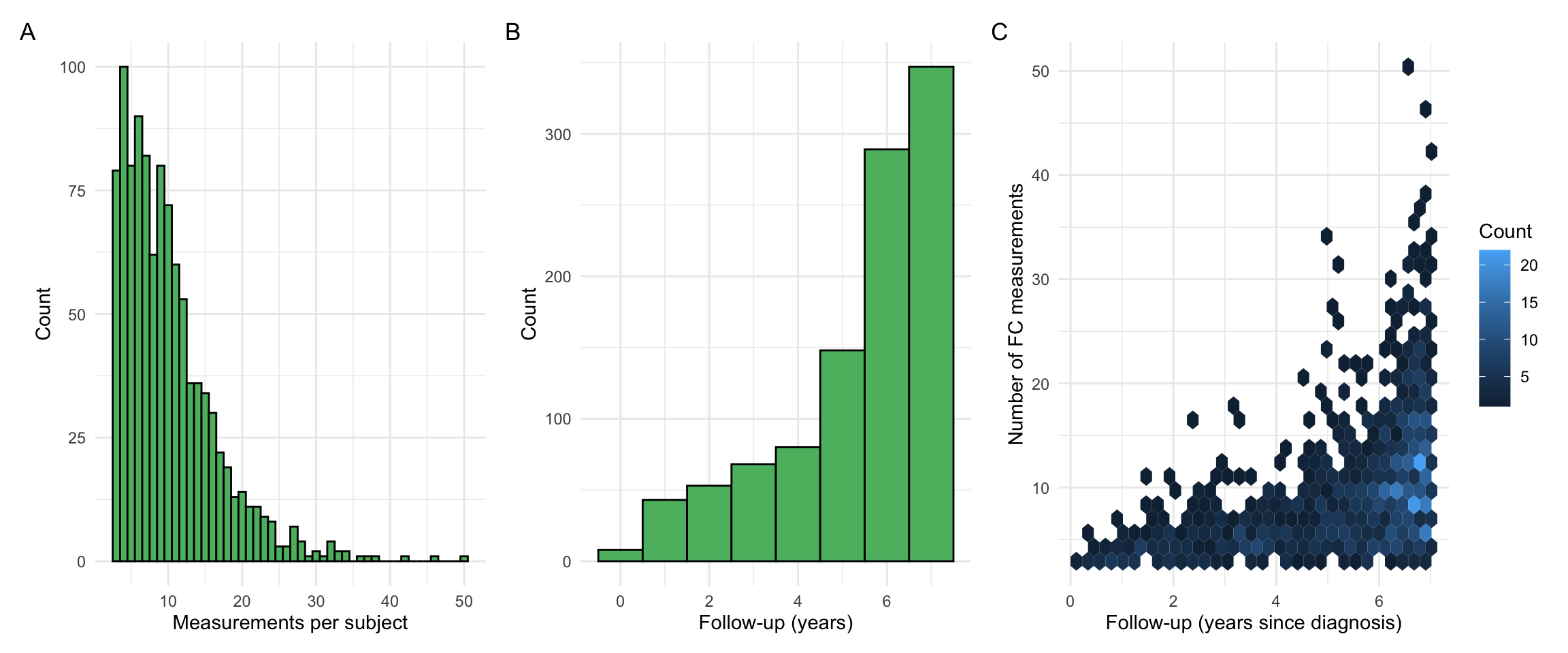
Revisiting month of diagnosis
After filtering by subjects who have a diagnostic FC available, January is no longer over-represented for month of diagnosis as we hypothesised (Figure 10)
Code
C-reactive protein
Code
crp <- crp[, c("ids", "COLLECTION_DATE", "TEST_DATA")] %>%
  subset(ids %in% dict$ids)

# Collection dates include collection times which are not required. Discarding.
crp$COLLECTION_DATE <- readr::parse_date(
  stringr::str_split_fixed(crp$COLLECTION_DATE, " ", n = 2)[, 1],
  format = "%Y-%m-%d"
)

colnames(crp) <- c("ids", "crp_date", "crp_result")

crp <- merge(crp,
  dict[, c("ids", "diagnosis")],
  by = "ids",
  all.x = TRUE
)
C-reactive protein (CRP) is a blood-based marker of inflammation. Unlike FCAL, which is highly specific to gastrointestinal inflammation, CRP levels are indicative of overall inflammation and are more likely to be affected by extra-intestinal factors such as infections. However, patient adherence to CRP testing is very strong, and CRP has seen historic usage in the field of IBD. Although CRP has been used for many years, we unfortunately only have test results from as early as 2008 due to the transition towards using TRAK for storing CRP results instead of the previous system.
As there is only one extract for CRP data (obtained from TRAK), merging multiple datasets is not required. As with the FCAL data, the recorded time of day for each test has been discarded in favour of the date. Any potential duplicate results have been removed.
Pre-processing of test results
Code
crp$crp_result <- as.numeric(
  plyr::mapvalues(
    crp$crp_result,
    from = c(
      "<0.2", "<1", "<1.", "<1.0", "<2", "<3", "<3.0", "<5",
      ">90", ">320"
    ),
    to = c(1, 1, 1, 1, 2, 3, 3, 5, 90, 320)
  )
)

# Lower-bound censoring
crp <- crp %>%
  mutate(crp_result = if_else(crp_result < 1, 1, crp_result))

# Remove error test results
crp <- crp[!is.na(crp[, "crp_result"]), ]
# Map numerical <1 test results (e.g 0.2) to 1.
CRP is left-censored, but does not appear to be right-censored. Multiple cut-offs are reported (1.1, 1.6, 2, 3, 3.5, 4, 5) with there also being variations for how < 1mg/L is reported (1.6, 2, 3). We map every observation < 1 to 1 and map <2, <3, and < 5 to 2, 3, and 5 respectively. Any failed tests (e.g due to contamination or an insufficient sample being provided) are discarded. As such, 1mg/L is used as a left censoring value for CRP.
As can be seen in Figure 11, extremely elevated CRP has been observed in some cases. These observations are physiologically valid. However, these data may skew our models and may be candidates for removal.
Code
crp %>%
  ggplot(aes(x = crp_result)) +
  geom_density(
    linewidth = 0.8,
    alpha = 0.5,
    fill = "#FFC800",
    color = "#FF8427"
  ) +
  theme_minimal() +
  theme(axis.text.y = element_blank()) +
  xlab("CRP (mg/L)") +
  ylab("Density")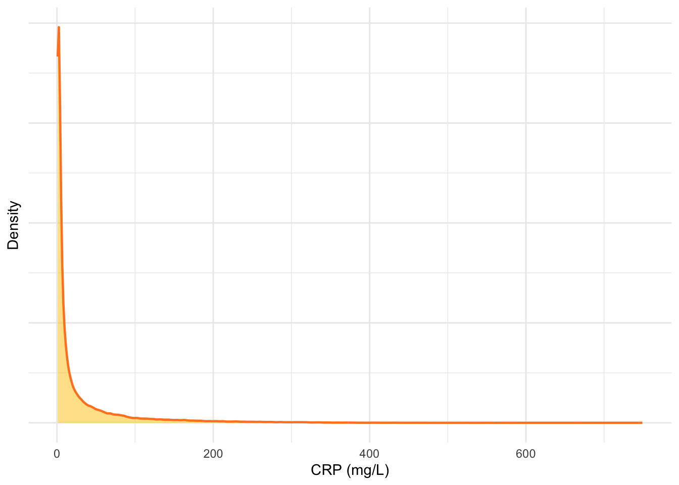
As with the FC data, the CRP data is also log transformed (Figure 12).
Code
crp %>%
  ggplot(aes(x = log(crp_result))) +
  geom_density(
    linewidth = 0.8,
    alpha = 0.5,
    fill = "#FFC800",
    color = "#FF8427"
  ) +
  theme_minimal() +
  theme(axis.text.y = element_blank()) +
  xlab("log(CRP (mg/L))") +
  ylab("Density")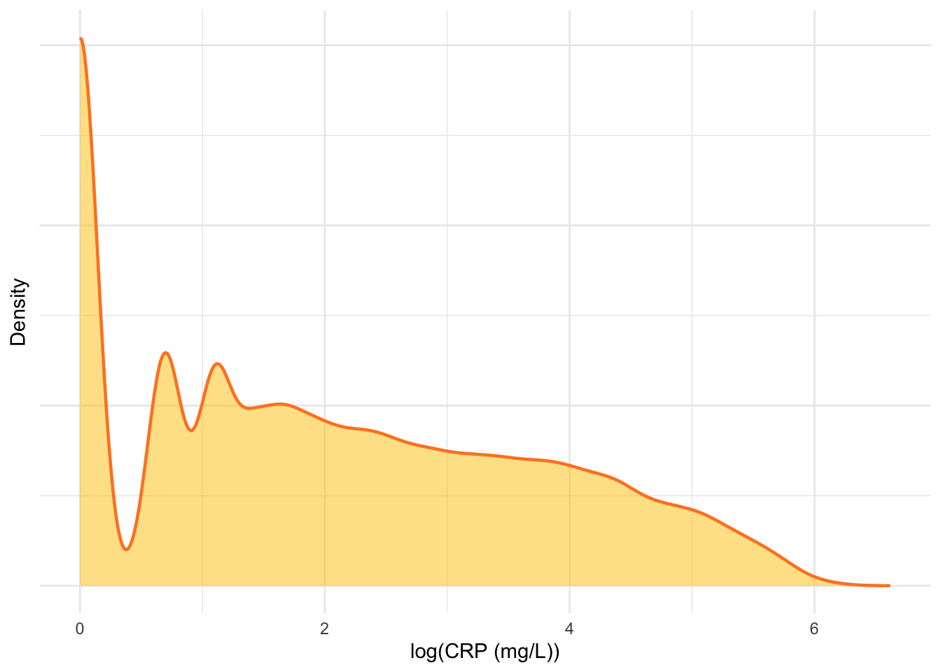
Observing Figure 12, it would appear the influence of extremely elevated CRP results will be minimal.
Removal of duplicates
As multiple CRP measurements are possible within a short time-frame, we only consider as duplicates those with an exact match by ids, crp_date and crp_result.
Retiming - part 1
As with the FCAL data, the times of CRP measurements are retimed and scaled to be the number of years since IBD diagnosis.
Code
crp <- merge(crp, dict[, c("ids", "date.of.diag")],
  by = "ids", all.x = TRUE, all.y = FALSE
)

# Dates have already been converted to Date class by fix_date_char() for dict
crp$crp_time <- as.numeric(crp$crp_date - crp$date.of.diag) / 365.25

crp %>%
  ggplot(aes(x = crp_time, y = log(crp_result), color = factor(ids))) +
  geom_line(alpha = 0.2) +
  geom_point(alpha = 0.3) +
  theme_minimal() +
  scale_color_manual(values = viridis::viridis(length(unique(crp$ids)))) +
  guides(color = "none") +
  xlab("Time (years)") +
  ylab("Log(CRP (mg/L))") +
  ggtitle("")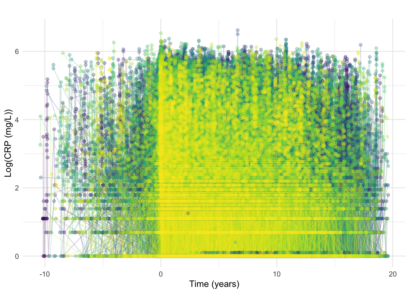
As should be expected given the ubiquitous nature of CRP testing, many CRP observations are earlier than diagnosis (Figure 13). Tests taken close to reported date of diagnosis are likely “early” as a result of diagnostic delay whereas tests from much earlier were likely requested due to other conditions.
As with FCAL, CRP results earlier than 90 days prior to diagnosis will be discarded. If a subject has a CRP within 90 days before diagnosis, then all of their CRP tests will be retimed such that their earliest CRP within this period is equal to 0 and all later measurements are shifted accordingly to maintain the same differences between measurement times.
This may mean t_0 corresponds to slightly different dates across FCAL and CRP for the same subject.
We also reduce the dataset to only subjects with a diagnostic CRP which equates to subjects with a CRP measurement within 3 months of diagnosis t \leq 0.25
Code
crp <- subset(crp, crp_time >= -0.25)Inclusion/exclusion: removal of subjects without a diagnostic CRP test
As indicated in our inclusion/exclusion criteria, we reduce the dataset to only subjects with a diagnostic FC. This equates to subjects with at least one FCAL measurement within 3 months of diagnosis t \leq 0.25.
After this exclusion, 2406 remain in the data.
Code
diag.time <- c()
crp.ids <-  unique(crp$ids)

for (id in crp.ids) {
  temp <- subset(crp, ids == id)
  temp <- temp[order(temp$crp_time), ]
  diag.time <- c(diag.time, temp[1, "crp_time"])
}


crp.dist <- data.frame(ids = crp.ids, diagnostic = diag.time)

saveRDS(crp.dist, paste0(prefix, "processed/crp-diag-dist.RDS"))606 subjects which were excluded due to not having a diagnostic crp had a reported date of diagnosis of 1st January.
Retiming - part 2
Here, we show the distribution of the diagnostic CRP measurements with respect to diagnosis date (in days).
Code
p <- crp %>%
  group_by(ids) %>%
  filter(crp_time == min(crp_time)) %>%
  ggplot(aes(x = crp_time * 365.25)) +
  geom_density(fill = "#415A77", color = "#1B263B") +
  theme_minimal() +
  labs(
    y = "Density",
    x = "Time from diagnosis to first CRP (days)"
  ) +
  geom_vline(xintercept = 0, linetype = "dashed", color = "red")

ggsave("plots/crp-diagnostic-dist.png",
  p,
  width = 16 * 2 / 3,
  height = 6,
  units = "in"
)
Similar to what was observed for FC, most diagnostic measurements were around the recorded diagnosis time (near zero). Here, we also retime measurements/diagnosis time as described above (i.e. time = 0 matches the time of first available CRP measurement). This is only applied to individuals for which the first available CRP is prior to the recorded diagnosis time.
Code
[1] 2406Code
crp %>%
  ggplot(aes(x = crp_time, y = log(crp_result), color = factor(ids))) +
  geom_line(alpha = 0.2) +
  geom_point(alpha = 0.3) +
  theme_minimal() +
  scale_color_manual(values = viridis::viridis(length(unique(crp$ids)))) +
  guides(color = "none") +
  xlab("Time (years)") +
  ylab("Log(CRP (mg/L))") +
  ggtitle("")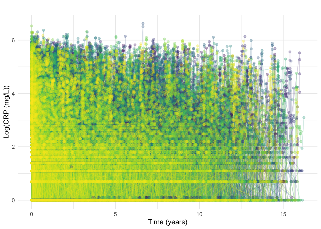
At this stage, we also exclude CRP measurements recorded beyond 7-years post diagnosis.
At this point, the data contains 10545 FCAL measurements across all 1036 individuals.
Additional pre-processing
Here, we summarise the number of observations per individual (with and without considering censored values) as well as length of follow-up. The latter is defined as the difference (in years) between diagnosis time and the time of the latest CRP measurement.
Code
countsDF <- crp %>%
  group_by(ids) %>%
  summarise(
    n.total = n(),
    censored.left = sum(crp_result == 1),
    n.noncensored = n.total - censored.left,
    n.negtime.nondiag = sum(crp_time != 0 & crp_date - date.of.diag < 0),
    followup = max(crp_time)
  )

p1 <- countsDF %>%
  ggplot(aes(x = n.total)) +
  geom_histogram(color = "black", fill = "#5BBA6F", binwidth = 1) +
  theme_minimal() +
  ylab("Count") +
  xlab("Measurements per subject")
p2 <- countsDF %>%
  ggplot(aes(x = followup)) +
  geom_histogram(color = "black", fill = "#5BBA6F", binwidth = 1) +
  theme_minimal() +
  ylab("Count") +
  xlab("Follow-up (years)")
p3 <- countsDF %>%
  ggplot(aes(y = n.total, x = followup)) +
  geom_hex() +
  xlab("Follow-up (years since diagnosis)") +
  ylab("Number of CRP measurements") +
  theme_minimal() +
  labs(fill = "Count")

p1 + p2 + p3 + plot_annotation(tag_levels = "A")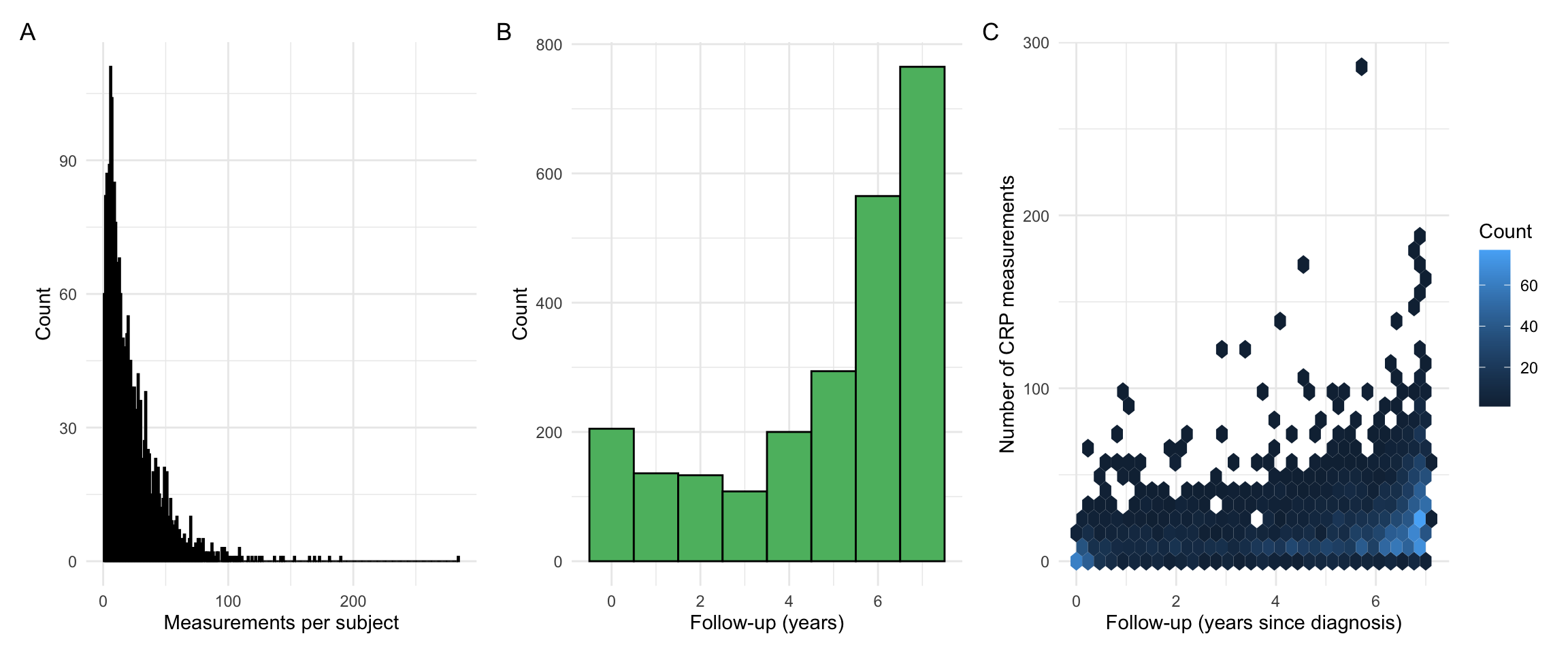
Our observations are very similar to what we had for FCAL. However, as CRP measurement frequency is higher, we find a lower proportion of individuals with a low follow-up time.
As CRP is not specific to gastrointestinal inflammation, a variety of factors (e.g. infection) can affect the measurements. To focus on long-term trends, further processing was applied to smooth out short-term fluctuations. Measurements were grouped into intervals of t: [0, 0.5), [0.5, 1.5), [1.5, 2.5), [2.5, 3.5), [3.5, 4.5), [4.5, 5.5), [5.5, 7], where t = 0 (years) is the time of diagnosis. The median CRP for each interval was calculated for each subject and used as input for subsequent analyses. The centre of each interval was used as the corresponding observation time.
Code
id.list <- unique(crp$ids)
crp.ma <- matrix(NA, nrow = length(id.list), ncol = 7)

for (i in seq_along(id.list)) {
  subject_data <- subset(crp, ids == id.list[i])
  for (j in seq(0, 6)) {
    if (j == 6) {
      sub.obs <- subset(
        subject_data,
        crp_time >= j - 0.5 & crp_time <= j + 1
      )
    } else {
      sub.obs <- subset(
        subject_data,
        crp_time >= j - 0.5 & crp_time < j + 0.5
      )
    }
    if (nrow(sub.obs) > 0) {
      crp.ma[i, j + 1] <- median(sub.obs$crp_result)
    }
  }
}
rownames(crp.ma) <- id.list

# Convert back to a long-format dataset and rename columns
crp.ma <- reshape2::melt(t(crp.ma), id.vars = row.names(crp.ma), na.rm = TRUE)
colnames(crp.ma) <- c("crp_time", "ids", "crp_result")
crp.ma <- crp.ma[, c(2, 3, 1)]

# Reset the time to start at zero
crp.ma$crp_time <- crp.ma$crp_time - 1

# Take into account uneven spacing at start and end
crp.ma$crp_time <- plyr::mapvalues(crp.ma$crp_time,
  from = c(0, 6),
  to = c(0.25, 6.25)
)

# Add diagnosis type back
crp.ma <- merge(crp.ma, dict[, -3], by = "ids", all.x = TRUE, all.y = FALSE)
Inclusion/exclusion: a minimum number of CRP measurements
Note that our inclusion criteria requires at least 3 CRP measurements per individual. This is applied after the additional pre-processing applied in the previous section. Here, we re-calculate relevant summary statistics.
Code
countsDF <- crp.ma %>%
  group_by(ids) %>%
  summarise(
    n.total = n(),
    censored.left = sum(crp_result == 0), # 0 because it was log transformed
    n.noncensored = n.total - censored.left,
    followup = max(crp_time),
    crp.var = var(crp_result, na.rm = TRUE)
  )

p1 <- countsDF %>%
  ggplot(aes(x = n.total)) +
  geom_histogram(color = "black", fill = "#5BBA6F", binwidth = 1) +
  theme_minimal() +
  ylab("Count") +
  xlab("Measurements per subject")
p2 <- countsDF %>%
  ggplot(aes(x = followup)) +
  geom_histogram(color = "black", fill = "#5BBA6F", binwidth = 1) +
  theme_minimal() +
  ylab("Count") +
  xlab("Follow-up (years)")
p3 <- countsDF %>%
  ggplot(aes(y = n.total, x = followup)) +
  geom_hex() +
  xlab("Follow-up (years since diagnosis)") +
  ylab("Number of CRP measurements") +
  theme_minimal() +
  labs(fill = "Count")

p1 + p2 + p3 + plot_annotation(tag_levels = "A")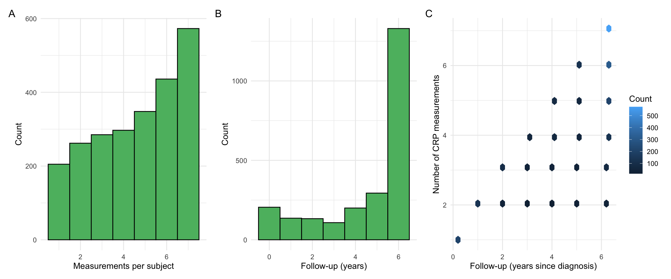
Code
# Number of individuals with at least 3 CRP measurements
sum(countsDF$n.total >= 3)
[1] 1939Code
# Number of individuals with at least 3 CRP measurements and non zero variance
sum(countsDF$n.total >= 3 & countsDF$crp.var != 0)
[1] 1838Code
# Number of individuals with at least 3 non-censored FCAL measurements
sum(countsDF$n.noncensored >= 3)
[1] 1939The following is used to select individuals with at least 3 CRP measurements and non-zero variance.
This leaves a cohort with 1838 individuals.
Code
p1 <- countsDF %>%
  subset(n.total >= 3 & crp.var != 0) %>%
  ggplot(aes(x = n.total)) +
  geom_histogram(color = "black", fill = "#5BBA6F", binwidth = 1) +
  theme_minimal() +
  ylab("Count") +
  xlab("Measurements per subject")
p2 <- countsDF %>%
  subset(n.total >= 3 & crp.var != 0) %>%
  ggplot(aes(x = followup)) +
  geom_histogram(color = "black", fill = "#5BBA6F", binwidth = 1) +
  theme_minimal() +
  ylab("Count") +
  xlab("Follow-up (years)")
p3 <- countsDF %>%
  subset(n.total >= 3 & crp.var != 0) %>%
  ggplot(aes(y = n.total, x = followup)) +
  geom_point(color = "#FF4F79", size = 2) +
  xlab("Follow-up (years since diagnosis)") +
  ylab("Number of FCAL measurements") +
  theme_minimal() +
  geom_hline(yintercept = 3)

p1 + p2 + p3 + plot_annotation(tag_levels = "A")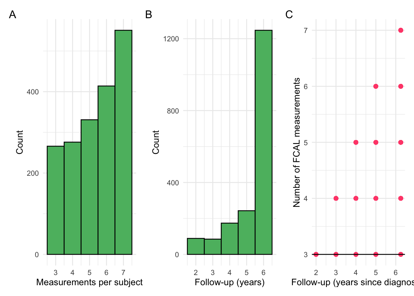
Additional pre-processing
Some subjects have the same median log-transformed CRP across all of their observations, effectively having a variance of 0. These subjects will be extracted and considered as their own cluster, as they may cause numerical issues when model fitting but remain of note.
Code
p1 <- crp.ma %>%
  ggplot(aes(x = crp_result)) +
  geom_density(
    linewidth = 0.8,
    alpha = 0.5,
    fill = "#EE92C2",
    color = "#7B5D6F"
  ) +
  theme_minimal() +
  theme(axis.text.y = element_blank()) +
  xlab("CRP (mg/L)") +
  ylab("Density")

p2 <- crp.ma %>%
  ggplot(aes(x = log(crp_result))) +
  geom_density(
    linewidth = 0.8,
    alpha = 0.5,
    fill = "#ADF1D2",
    color = "#50635A"
  ) +
  theme_minimal() +
  theme(axis.text.y = element_blank()) +
  xlab("log(CRP (mg/L))") +
  ylab("Density")

print(p1 + p2)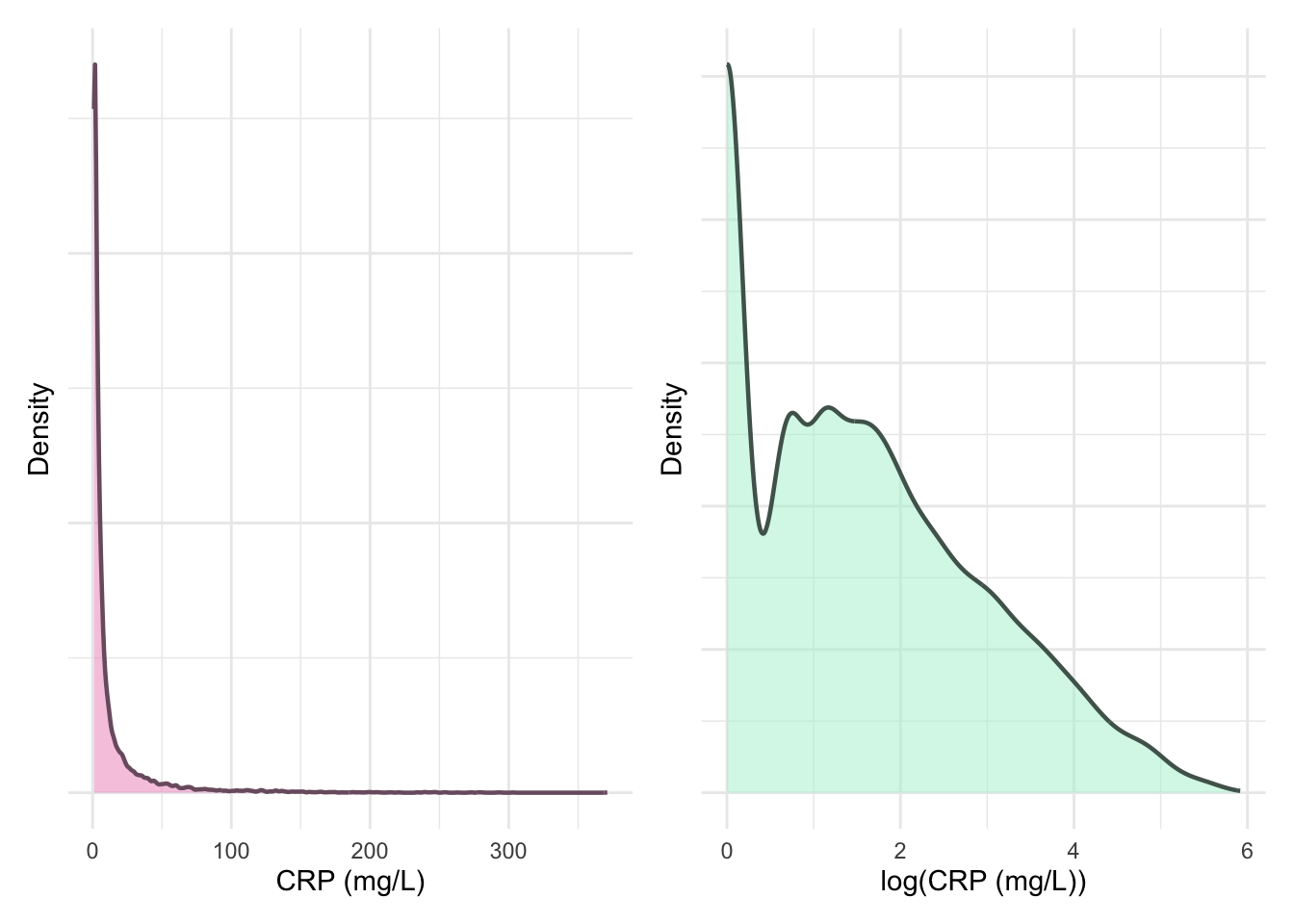
Code
ggsave("plots/crp-dist-ma.pdf", p1 + p2, width = 8, height = 4.5, units = "in")There are 9898 total data points after the additional preprocessing describing 1838 subjects.
25% 50% 75%
  4   6   7
Revisiting month of diagnosis
After filtering by subjects who have a diagnostic CRP available, January is no longer over-represented for month of diagnosis. This is a comparable finding to FC (Figure 10).
Code

Updated density plots
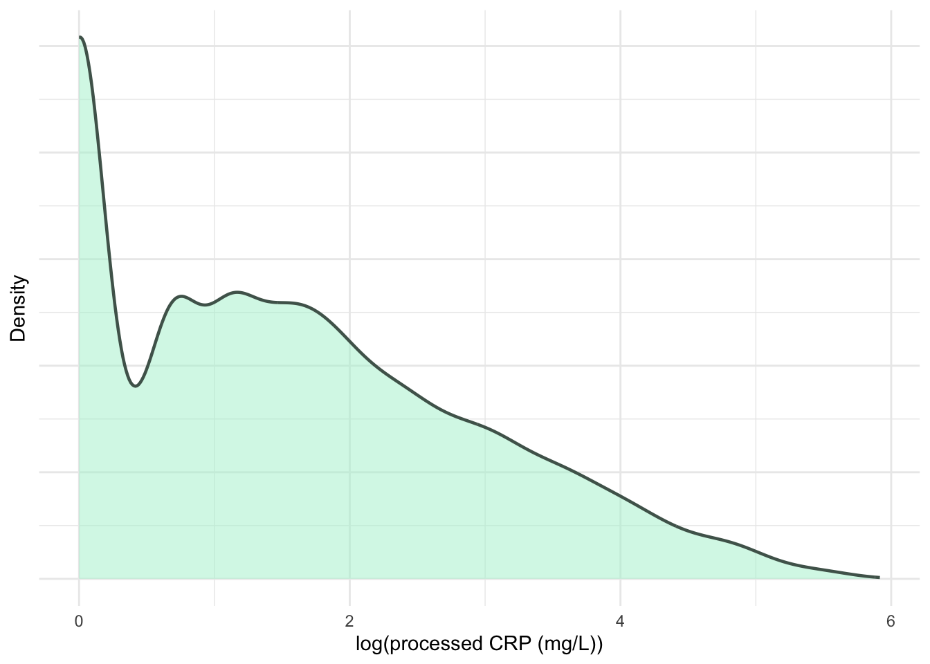
The following plots are updated versions of previous density plots (Figure 4, Figure 5, Figure 11 and Figure 12). These plots only include subjects who have met the inclusion criteria.
Code
p1 <- fcal %>%
  ggplot(aes(x = calpro_result)) +
  geom_density(
    linewidth = 0.8,
    alpha = 0.5,
    fill = "#2E86AB",
    color = "#07004D"
  ) +
  theme_minimal() +
  theme(axis.text.y = element_blank()) +
  xlab("FC (µg/g)") +
  ylab("Density")
print(p1)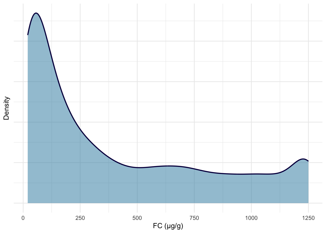
Code
p2 <- fcal %>%
  ggplot(aes(x = log(calpro_result))) +
  geom_density(
    linewidth = 0.8,
    alpha = 0.5,
    fill = "#F7A072",
    color = "#936136"
  ) +
  theme_minimal() +
  theme(axis.text.y = element_blank()) +
  xlab("log(FC (µg/g))") +
  ylab("Density")
print(p2)

ggsave("plots/fcal-dist.pdf", p1 + p2, width = 8, height = 4.5, units = "in")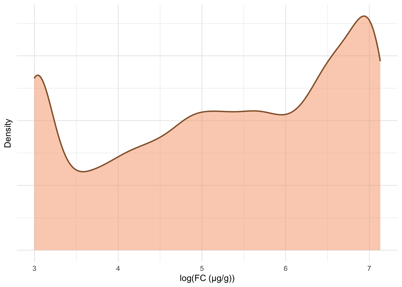
Code
p3 <- crp %>%
  ggplot(aes(x = crp_result)) +
  geom_density(
    linewidth = 0.8,
    alpha = 0.5,
    fill = "#EE92C2",
    color = "#7B5D6F"
  ) +
  theme_minimal() +
  theme(axis.text.y = element_blank()) +
  xlab("CRP (mg/L)") +
  ylab("Density")
print(p3)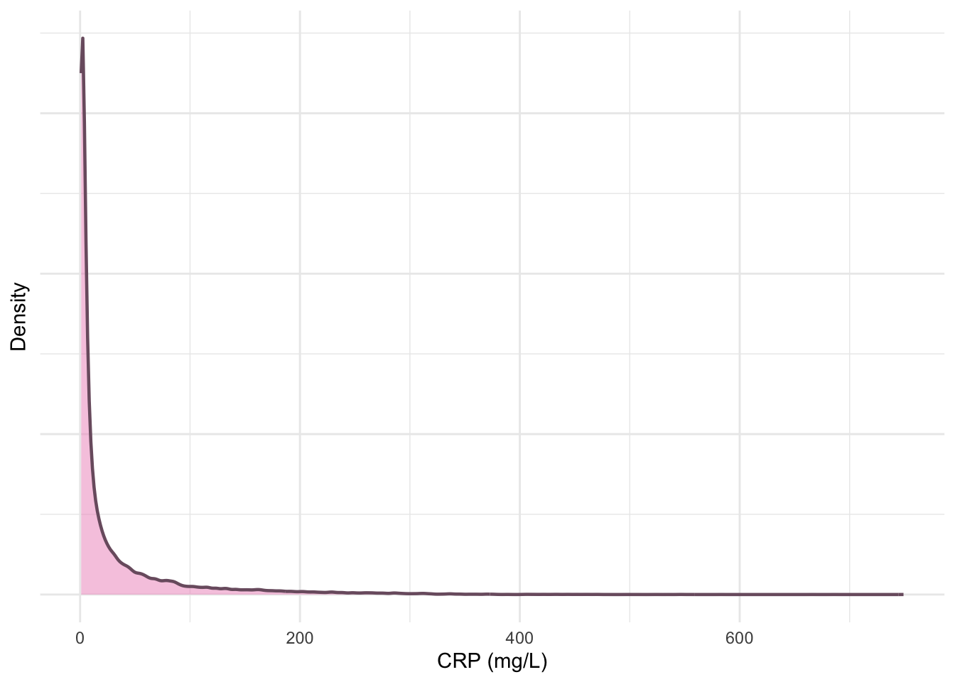
Code
p4 <- crp %>%
  ggplot(aes(x = log(crp_result))) +
  geom_density(
    linewidth = 0.8,
    alpha = 0.5,
    fill = "#ADF1D2",
    color = "#50635A"
  ) +
  theme_minimal() +
  theme(axis.text.y = element_blank()) +
  xlab("log(CRP (mg/L))") +
  ylab("Density")
print(p4)
ggsave("plots/crp-dist.pdf", p3 + p4, width = 8, height = 4.5, units = "in")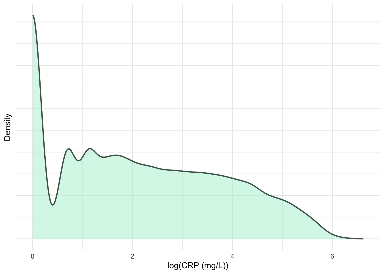
Code
p5 <- crp.ma %>%
  ggplot(aes(x = crp_result)) +
  geom_density(
    linewidth = 0.8,
    alpha = 0.5,
    fill = "#EE92C2",
    color = "#7B5D6F"
  ) +
  theme_minimal() +
  theme(axis.text.y = element_blank()) +
  xlab("Processed CRP (mg/L)") +
  ylab("Density")
print(p5)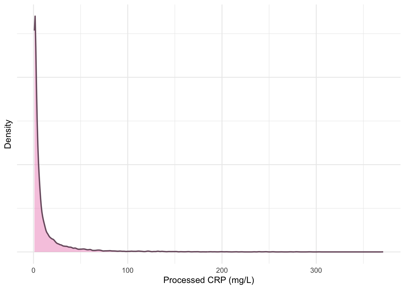
Code
p6 <- crp.ma %>%
  ggplot(aes(x = log(crp_result))) +
  geom_density(
    linewidth = 0.8,
    alpha = 0.5,
    fill = "#ADF1D2",
    color = "#50635A"
  ) +
  theme_minimal() +
  theme(axis.text.y = element_blank()) +
  xlab("log(processed CRP (mg/L))") +
  ylab("Density")
print(p6)
ggsave("plots/crp-processed-dist.pdf",
  p5 + p6,
  width = 8,
  height = 4.5,
  units = "in"
)


p <- (p1 + p2) / (p5 + p6) +
  plot_annotation(tag_levels = "A") &
  theme(plot.tag = element_text(size = 18, face = "bold"))


ggsave("plots/Sup-Figure-1.pdf",
  p,
  width = 8,
  height = 8,
  units = "in"
)
Code
25% 50% 75%
10 20 36 Data saving
The processed subject dictionary and FC and CRP datasets have been saved to files, so they can be used for the primary analysis.
Code
if (!dir.exists(paste0(prefix, "processed"))) {
  dir.create(paste0(prefix, "processed"))
}

fcal$calpro_result <- log(fcal$calpro_result)
crp.ma$crp_result <- log(crp.ma$crp_result)


saveRDS(dict, paste0(prefix, "processed/dict-initial.RDS"))
saveRDS(fcal, paste0(prefix, "processed/fcal.RDS"))
saveRDS(crp, paste0(prefix, "processed/crp.RDS"))
saveRDS(crp.ma, paste0(prefix, "processed/median-crp.RDS"))
Code
25% 50% 75%
6 9 14 Acknowledgments
This work is funded by the Medical Research Council & University of Edinburgh via a Precision Medicine PhD studentship (MR/N013166/1, to NC-C).
References
Reuse
Licensed by CC BY unless otherwise stated.


Session info
Code
R version 4.4.3 (2025-02-28)
Platform: aarch64-apple-darwin20
locale: en_GB.UTF-8||en_GB.UTF-8||en_GB.UTF-8||C||en_GB.UTF-8||en_GB.UTF-8
attached base packages: stats, graphics, grDevices, utils, datasets, methods and base
other attached packages: patchwork(v.1.3.0), datefixR(v.1.7.0), pander(v.0.6.6), knitr(v.1.49), lubridate(v.1.9.4), forcats(v.1.0.0), stringr(v.1.5.1), dplyr(v.1.1.4), purrr(v.1.0.4), readr(v.2.1.5), tidyr(v.1.3.1), tibble(v.3.2.1), ggplot2(v.3.5.1) and tidyverse(v.2.0.0)
loaded via a namespace (and not attached): viridis(v.0.6.5), generics(v.0.1.3), lattice(v.0.22-6), stringi(v.1.8.4), hms(v.1.1.3), digest(v.0.6.37), magrittr(v.2.0.3), evaluate(v.1.0.3), grid(v.4.4.3), timechange(v.0.3.0), fastmap(v.1.2.0), plyr(v.1.8.9), jsonlite(v.1.9.1), gridExtra(v.2.3), viridisLite(v.0.4.2), scales(v.1.3.0), textshaping(v.1.0.0), cli(v.3.6.4), rlang(v.1.1.5), munsell(v.0.5.1), withr(v.3.0.2), yaml(v.2.3.10), tools(v.4.4.3), parallel(v.4.4.3), reshape2(v.1.4.4), tzdb(v.0.4.0), colorspace(v.2.1-1), vctrs(v.0.6.5), R6(v.2.6.1), lifecycle(v.1.0.4), htmlwidgets(v.1.6.4), ragg(v.1.3.3), pkgconfig(v.2.0.3), hexbin(v.1.28.5), pillar(v.1.10.1), gtable(v.0.3.6), glue(v.1.8.0), Rcpp(v.1.0.14), systemfonts(v.1.2.1), xfun(v.0.51), tidyselect(v.1.2.1), farver(v.2.1.2), htmltools(v.0.5.8.1), rmarkdown(v.2.29), labeling(v.0.4.3) and compiler(v.4.4.3)